16.4 A worked example: plot.advanced()
Let’s create our own advanced own custom plotting function called plot.advanced() that acts like the normal plotting function, but has several additional arguments
1 add.mean: A logical value indicating whether or not to add vertical and horizontal lines at the mean value of x and y. 2 add.regression: A logical value indicating whether or not to add a linear regression line 3 p.threshold: A numeric scalar indicating the p.value threshold for determining significance 4 add.modeltext: A logical value indicating whether or not to include the regression equation as a sub-title to the plot
This plotting code is a bit long, but it’s all stuff you’ve learned before.
plot.advanced <- function (x = rnorm(100),
                           y = rnorm(100),
                           add.mean = FALSE,
                           add.regression = FALSE,
                           p.threshold = .05,
                           add.modeltext = FALSE,
                           ...  # Optional further arguments passed on to plot
                           ) {

# Generate the plot with optional arguments
#   like main, xlab, ylab, etc.
  plot(x, y, ...)

# Add mean reference lines if add.mean is TRUE
if(add.mean == TRUE) {

  abline(h = mean(y), lty = 2)
  abline(v = mean(x), lty = 2)
}

# Add regression line if add.regression is TRUE
if(add.regression == TRUE) {

  model <- lm(y ~ x)  # Run regression

  p.value <- anova(model)$"Pr(>F)"[1] # Get p-value

  # Define line color from model p-value and threshold
  if(p.value < p.threshold) {line.col <- "red"}
  if(p.value >= p.threshold) {line.col <- "black"}

  abline(lm(y ~ x), col = line.col, lwd = 2) # Add regression line

}

  # Add regression equation text if add.modeltext is TRUE
if(add.modeltext == TRUE) {

  # Run regression
  model <- lm(y ~ x)

  # Determine coefficients from model object
  coefficients <- model$coefficients
  a <- round(coefficients[1], 2)
  b <- round(coefficients[2], 2)

  # Create text
  model.text <- paste("Regression Equation: ", a, " + ",
                      b, " * x", sep = "")

  # Add text to top of plot
  mtext(model.text, side = 3, line = .5, cex = .8)

}
}
Let’s try it out!
plot.advanced(x = pirates$age,
              y = pirates$tchests,
              add.regression = TRUE,
              add.modeltext = TRUE,
              p.threshold = .05,
              main = "plot.advanced()",
              xlab = "Age", ylab = "Treasure Chests Found",
              pch = 16,
              col = gray(.2, .3))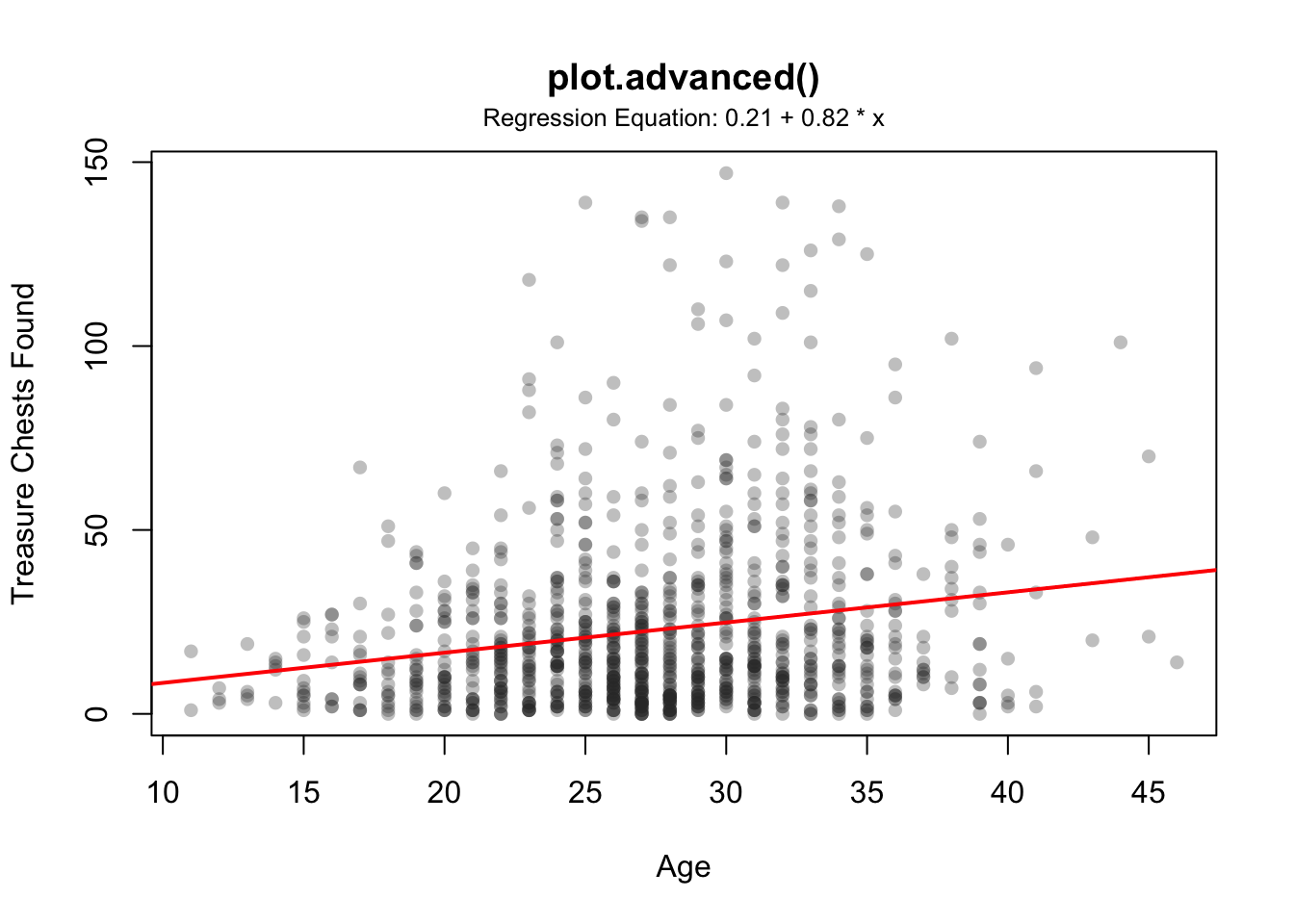
16.4.1 Seeing function code
Because R is awesome, you can view the code underlying most functions by just evaluating the name of the function (without any parentheses or arguments). For example, the yarrr package contains a function called transparent() that converts standard colors into transparent colors. To see the code contained in the function, just evaluate its name:
# Show me the code in the transparent() function
transparent
## function (orig.col = "red", trans.val = 1, maxColorValue = 255)
## {
##     n.cols <- length(orig.col)
##     orig.col <- col2rgb(orig.col)
##     final.col <- rep(NA, n.cols)
##     for (i in 1:n.cols) {
##         final.col[i] <- rgb(orig.col[1, i], orig.col[2, i], orig.col[3,
##             i], alpha = (1 - trans.val) * 255, maxColorValue = maxColorValue)
##     }
##     return(final.col)
## }
## <bytecode: 0x1127bb108>
## <environment: namespace:yarrr>
Once you know the code underlying a function, you can easily copy it and edit it to your own liking. Or print it and put it above your bed. Totally up to you.
16.4.2 Using stop() to completely stop a function and print an error
By default, all the code in a function will be evaluated when it is executed. However, there may be cases where there’s no point in evaluating some code and it’s best to stop everything and leave the function altogether. For example, let’s say you have a function called do.stats() that has a single argument called mat which is supposed to be a matrix. If the user accidentally enters a dataframe rather than a matrix, it might be best to stop the function altogether rather than to waste time executing code. To tell a function to stop running, use the stop() function.
If R ever executes a stop() function, it will automatically quit the function it’s currently evaluating, and print an error message. You can define the exact error message you want by including a string as the main argument.
For example, the following function do.stats will print an error message if the argument mat is not a matrix.
do.stats <- function(mat) {

if(is.matrix(mat) == F) {stop("Argument was not a matrix!")}

# Only run if argument is a matrix!
print(paste("Thanks for giving me a matrix. The matrix has ", nrow(mat),
" rows and ", ncol(mat),
" columns. If you did not give me a matrix, the function would have stopped by now!",
sep = ""))

}
Let’s test it. First I’ll enter an argument that is definitely not a matrix:
do.stats(mat = "This is a string, not a matrix") Now I’ll enter a valid matrix argument:
do.stats(mat = matrix(1:10, nrow = 2, ncol = 5))
## [1] "Thanks for giving me a matrix. The matrix has 2 rows and 5 columns. If you did not give me a matrix, the function would have stopped by now!"
16.4.3 Using vectors as arguments
You can use any kind of object as an argument to a function. For example, we could re-create the function oh.god.how.much.did.i.spend by having a single vector object as the argument, rather than three separate values. In this version, we’ll extract the values of a, b and c using indexing:
oh.god.how.much.did.i.spend <- function(drinks.vec) {

  grogg <- drinks.vec[1]
  port <- drinks.vec[2]
  crabjuice <- drinks.vec[3]

  output <- grogg * 1 + port * 3 + crabjuice * 10

  return(output)

}
To use this function, the pirate will enter the number of drinks she had as a single vector with length three rather than as 3 separate scalars.
oh.god.how.much.did.i.spend(c(1, 5, 2))
## [1] 36
16.4.4 Storing and loading your functions to and from a function file with source()
As you do more programming in R, you may find yourself writing several function that you’ll want to use again and again in many different R scripts. It would be a bit of a pain to have to re-type your functions every time you start a new R session, but thankfully you don’t need to do that. Instead, you can store all your functions in one R file and then load that file into each R session.
I recommend that you put all of your custom R functions into a single R script with a name like customfunctions.R. Mine is called Custom_Pirate_Functions.R. Once you’ve done this, you can load all your functions into any R session by using the source() function. The source function takes a file directory as an argument (the location of your custom function file) and then executes the R script into your current session.
For example, on my computer my custom function file is stored at Users/Nathaniel/Dropbox/Custom_Pirate_Functions.R. When I start a new R session, I load all of my custom functions by running the following code:
# Evaluate all of the code in my custom function R script
source(file = "Users/Nathaniel/Dropbox/Custom_Pirate_Functions.R")
Once I’ve run this, I have access to all of my functions, I highly recommend that you do the same thing!
16.4.5 Testing functions
When you start writing more complex functions, with several inputs and lots of function code, you’ll need to constantly test your function line-by-line to make sure it’s working properly. However, because the input values are defined in the input definitions (which you won’t execute when testing the function), you can’t actually test the code line-by-line until you’ve defined the input objects in some other way. To do this, I recommend that you include temporary hard-coded values for the inputs at the beginning of the function code.
For example, consider the following function called remove.outliers. The goal of this function is to take a vector of data and remove any data points that are outliers. This function takes two inputs x and outlier.def, where x is a vector of numerical data, and outlier.def is used to define what an outlier is: if a data point is outlier.def standard deviations away from the mean, then it is defined as an outlier and is removed from the data vector.
In the following function definition, I’ve included two lines where I directly assign the function inputs to certain values (in this case, I set x to be a vector with 100 values of 1, and one outlier value of 999, and outlier.def to be 2). Now, if I want to test the function code line by line, I can uncomment these test values, execute the code that assigns those test values to the input objects, then run the function code line by line to make sure the rest of the code works.
remove.outliers <- function(x, outlier.def = 2) {

# Test values (only used to test the following code)
#  x <- c(rep(1, 100), 999)
#  outlier.def <- 2

  is.outlier <- x > (mean(x) + outlier.def * sd(x)) |
                x < (mean(x) - outlier.def * sd(x))

  x.nooutliers <- x[is.outlier == FALSE]

  return(x.nooutliers)

}
Trust me, when you start building large complex functions, hard-coding these test values will save you many headaches. Just don’t forget to comment them out when you are done testing or the function will always use those values!
16.4.6 Using ... as a wildcard argument
For some functions that you write, you may want the user to be able to specify inputs to functions within your overall function. For example, if I create a custom function that includes the histogram function hist() in R, I might also want the user to be able to specify optional inputs for the plot, like main, xlab, ylab, etc. However, it would be a real pain in the pirate ass to have to include all possible plotting parameters as inputs to our new function. Thankfully, we can take care of all of this by using the ... notation as an input to the function. Note that the ... notation will only pass arguments on to functions that are specifically written to allow for optional inputs. If you look at the help menu for hist(), you’ll see that it does indeed allow for such option inputs passed on from other functions. The ... input tells R that the user might add additional inputs that should be used later in the function.
Here’s a quick example, let’s create a function called hist.advanced() that plots a histogram with some optional additional arguments passed on with ...
hist.advanced <- function(x, add.ci = TRUE, ...) {

hist(x, # Main Data
     ... # Here is where the additional arguments go
     )

if(add.ci == TRUE) {

  ci <- t.test(x)$conf.int # Get 95% CI
  segments(ci[1], 0, ci[2], 0, lwd = 5, col = "red")

  mtext(paste("95% CI of Mean = [", round(ci[1], 2), ",",
              round(ci[2], 2), "]"), side = 3, line = 0)
}
}
Now, let’s test our function with the optional inputs main, xlab, and col. These arguments will be passed down to the hist() function within hist.advanced(). Here is the result:
hist.advanced(x = rnorm(100), add.ci = TRUE,
              main = "Treasure Chests found",
              xlab = "Number of Chests",
              col = "lightblue")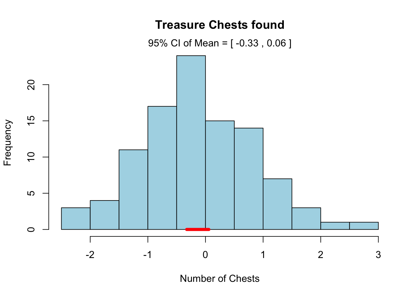
As you can see, R has passed our optional plotting arguments down to the main hist() function in the function code.