5.4 Local likelihood

We next explore an extension of the local polynomial estimator that imitates the expansion that generalized linear models made of linear models, allowing the former to consider non-continuous responses. This extension is aimed to estimate the regression function by relying on the likelihood, rather than the least squares. The main idea behind local likelihood is, therefore, to locally fit parametric models by maximum likelihood.

We begin by seeing that local likelihood based on the linear model is equivalent to local polynomial modeling. Theorem B.1 shows that, under the assumptions given in Section B.1.2, the maximum likelihood estimate of $\boldsymbol{\beta}$ in the linear model

$$\begin{align} Y|(X_1,\ldots,X_p)\sim\mathcal{N}(\beta_0+\beta_1X_1+\cdots+\beta_pX_p,\sigma^2)\tag{5.15} \end{align}$$

is equivalent to the least squares estimate, $\hat{\boldsymbol{\beta}}=(\mathbf{X}'\mathbf{X})^{-1}\mathbf{X}'\mathbf{Y}.$ The reason for this is the form of the conditional (on $X_1,\ldots,X_p$) log-likelihood:

$$\begin{align*} \ell(\boldsymbol{\beta})=&-\frac{n}{2}\log(2\pi\sigma^2)\nonumber\\ &-\frac{1}{2\sigma^2}\sum_{i=1}^n(Y_i-\beta_0-\beta_1X_{i1}-\cdots-\beta_pX_{ip})^2. \end{align*}$$

If there is a single predictor $X,$ the situation on which we focus on, a polynomial fitting of order $p$ of the conditional mean can be achieved by the well-known trick of identifying the $j$-th predictor $X_j$ in (5.15) by $X^j.$¹⁸⁸ This results in

$$\begin{align} Y|X\sim\mathcal{N}(\beta_0+\beta_1X+\cdots+\beta_pX^p,\sigma^2).\tag{5.16} \end{align}$$

Therefore, we can define the weighted log-likelihood of the linear model (5.16) about $x$ as

$$\begin{align} \ell_{x,h}(\boldsymbol{\beta}):=& -\frac{n}{2}\log(2\pi\sigma^2)\tag{5.17}\\ &-\frac{1}{2\sigma^2}\sum_{i=1}^n(Y_i-\beta_0-\beta_1(X_i-x)-\cdots-\beta_p(X_i-x)^p)^2K_h(x-X_i).\nonumber \end{align}$$

Maximizing with respect to $\boldsymbol{\beta}$ the local log-likelihood (5.17) provides $\hat\beta_0=\hat{m}(x;p,h),$ which is precisely the local polynomial estimator, as it was obtained in (4.10), but now obtained from a likelihood-based perspective. The key point is to realize that the very same idea can be applied to the family of generalized linear models, for which linear regression (in this case manifested as a polynomial regression) is just a particular case.

Figure 5.1: Construction of the local likelihood estimator. The animation shows how local likelihood fits in a neighborhood of $x$ are combined to provide an estimate of the regression function for binary response, which depends on the polynomial degree, bandwidth, and kernel (gray density at the bottom). The data points are shaded according to their weights for the local fit at $x.$ Application available here.

We illustrate the local likelihood principle for the logistic regression (see Section B.2 for a quick review). In this case, the sample is $(X_1,Y_1),\ldots,(X_n,Y_n)$ with

$$\begin{align*} Y_i|X_i\sim \mathrm{Ber}(\mathrm{logistic}(\eta(X_i))),\quad i=1,\ldots,n, \end{align*}$$

with the polynomial term¹⁸⁹

$$\begin{align*} \eta(x):=\beta_0+\beta_1x+\cdots+\beta_px^p. \end{align*}$$

The log-likelihood of $\boldsymbol{\beta}$ is

$$\begin{align*} \ell(\boldsymbol{\beta})=&\,\sum_{i=1}^n\left\{Y_i\log(\mathrm{logistic}(\eta(X_i)))+(1-Y_i)\log(1-\mathrm{logistic}(\eta(X_i)))\right\}\nonumber\\ =&\,\sum_{i=1}^n\ell(Y_i,\eta(X_i)), \end{align*}$$

where we consider the log-likelihood addend $\ell(y,\eta):=y\eta-\log(1+e^\eta).$ For the sake of clarity in the next developments, we make explicit the dependence on $\eta(x)$ of this addend; conversely, we make its dependence on $\boldsymbol{\beta}$ implicit.

The local log-likelihood of $\boldsymbol{\beta}$ about $x$ is then defined as

$$\begin{align} \ell_{x,h}(\boldsymbol{\beta}):=\sum_{i=1}^n\ell(Y_i,\eta(X_i-x))K_h(x-X_i).\tag{5.18} \end{align}$$

Maximizing¹⁹⁰ the local log-likelihood (5.18) with respect to $\boldsymbol{\beta}$ provides

$$\begin{align*} \hat{\boldsymbol{\beta}}_{h}=\arg\max_{\boldsymbol{\beta}\in\mathbb{R}^{p+1}}\ell_{x,h}(\boldsymbol{\beta}). \end{align*}$$

The local likelihood estimate of $\eta(x)$ is the intercept of this fit,

$$\begin{align*} \hat\eta(x):=\hat\beta_{h,0}. \end{align*}$$

Note that the dependence of $\hat\beta_{h,0}$ on $x$ is omitted. From $\hat\eta(x),$ we can obtain the local logistic regression evaluated at $x$ as¹⁹¹

$$\begin{align} \hat{m}_{\ell}(x;p,h):=g^{-1}\left(\hat\eta(x)\right)=\mathrm{logistic}(\hat\beta_{h,0}).\tag{5.19} \end{align}$$

Each evaluation of $\hat{m}_{\ell}(x;p,h)$ in a different $x$ requires, thus, a weighted fit of the underlying local logistic model.

The code below shows three different ways of implementing in R the local logistic regression (with $p=1$).

# Simulate some data
n <- 200
logistic <- function(x) 1 / (1 + exp(-x))
p <- function(x) logistic(1 - 3 * sin(x))
set.seed(123456)
X <- sort(runif(n = n, -3, 3))
Y <- rbinom(n = n, size = 1, prob = p(X))

# Set bandwidth and evaluation grid
h <- 0.25
x <- seq(-3, 3, l = 501)

# Approach 1: optimize the weighted log-likelihood through the workhorse
# function underneath glm, glm.fit
suppressWarnings(
  fit_glm <- sapply(x, function(x) {
    K <- dnorm(x = x, mean = X, sd = h)
    glm.fit(x = cbind(1, X - x), y = Y, weights = K,
            family = binomial())$coefficients[1]
  })
)

# Approach 2: optimize directly the weighted log-likelihood
suppressWarnings(
  fit_nlm <- sapply(x, function(x) {
    K <- dnorm(x = x, mean = X, sd = h)
    nlm(f = function(beta) {
      -sum(K * (Y * (beta[1] + beta[2] * (X - x)) -
                  log(1 + exp(beta[1] + beta[2] * (X - x)))))
      }, p = c(0, 0))$estimate[1]
  })
)

# Approach 3: employ locfit::locfit
# CAREFUL: locfit::locfit uses a different internal parametrization for h!
# As it can be see, the bandwidths in approaches 1-2 and approach 3 do NOT
# give the same results! With h = 0.75 in locfit::locfit the fit is close
# to the previous ones (done for h = 0.25), but not exactly the same...
fit_locfit <- locfit::locfit(Y ~ locfit::lp(X, deg = 1, h = 0.75),
                             family = "binomial", kern = "gauss")

# Compare fits
plot(x, p(x), ylim = c(0, 1.5), type = "l", lwd = 2)
lines(x, logistic(fit_glm), col = 2, lwd = 2)
lines(x, logistic(fit_nlm), col = 3, lty = 2)
lines(x, predict(fit_locfit, newdata = x), col = 4)
legend("topright", legend = c("p(x)", "glm", "nlm", "locfit"),
       lwd = 2, col = c(1, 2, 3, 4), lty = c(1, 1, 2, 1))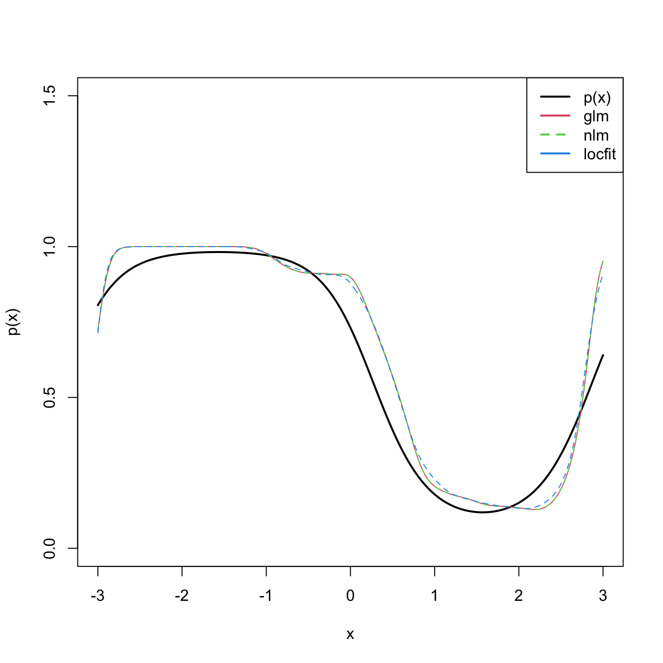

Bandwidth selection can be done by means of likelihood cross-validation. The objective is to maximize the local log-likelihood fit at $(X_i,Y_i)$ but removing the influence by the datum itself. That is,

$$\begin{align} \hat{h}_{\mathrm{LCV}}&=\arg\max_{h>0}\mathrm{LCV}(h),\nonumber\\ \mathrm{LCV}(h)&=\sum_{i=1}^n\ell(Y_i,\hat\eta_{-i}(X_i)),\tag{5.20} \end{align}$$

where $\hat\eta_{-i}(X_i)$ represents the local fit at $X_i$ without the $i$-th datum $(X_i,Y_i).$¹⁹² Unfortunately, the nonlinearity of (5.19) forbids a simplifying result as the one in Proposition 4.1. Thus, in principle, it is required to fit $n$ local likelihoods for sample size $n-1$ to obtain a single evaluation of (5.20).¹⁹³

We conclude by illustrating how to compute the LCV function and optimize it. Keep in mind that much more efficient implementations are possible!

# Exact LCV - recall that we *maximize* the LCV!
h <- seq(0.1, 2, by = 0.1)
suppressWarnings(
  LCV <- sapply(h, function(h) {
  sum(sapply(1:n, function(i) {
    K <- dnorm(x = X[i], mean = X[-i], sd = h)
    nlm(f = function(beta) {
      -sum(K * (Y[-i] * (beta[1] + beta[2] * (X[-i] - X[i])) -
                  log(1 + exp(beta[1] + beta[2] * (X[-i] - X[i])))))
      }, p = c(0, 0))$minimum
    }))
  })
)
plot(h, LCV, type = "o")
abline(v = h[which.max(LCV)], col = 2)

Exercise 5.12 (Adapted from Example 4.6 in Wasserman (2006)) The dataset at http://www.stat.cmu.edu/~larry/all-of-nonpar/=data/bpd.dat (alternative link) contains information about the presence of bronchopulmonary dysplasia (binary response) and the birth weight in grams (predictor) of $223$ newborns.

1. Use the three approaches described above to compute the local logistic regression (first degree) and plot their outputs for a bandwidth that is somehow adequate.
2. Using $\hat{h}_{\mathrm{LCV}},$ explore and comment on the resulting estimates, providing insights into the data.
3. From the obtained fit, derive several simple medical diagnostic rules for the probability of the presence of bronchopulmonary dysplasia from the birth weight.

Exercise 5.13 The challenger.txt dataset contains information regarding the state of the solid rocket boosters after launch for $23$ shuttle flights prior the Challenger launch. Each row has, among others, the variables fail.field (indicator of whether there was an incident with the O-rings), nfail.field (number of incidents with the O-rings), and temp (temperature in the day of launch, measured in Celsius degrees). See Section 5.1 in García-Portugués (2025) for further context on the Challenger case study.

1. Fit a local logistic regression (first degree) for fails.field ~ temp, for three choices of bandwidths: one that oversmooths, another that is somehow adequate, and another that undersmooths. Do the effects of temp on fails.field seem to be significant?
2. Obtain $\hat{h}_{\mathrm{LCV}}$ and plot the LCV function with a reasonable accuracy.
3. Using $\hat{h}_{\mathrm{LCV}},$ predict the probability of an incident at temperatures $-0.6$ (launch temperature of the Challenger) and $11.67$ (vice president of engineers’ recommended launch threshold).
4. What are the local odds at $-0.6,$ $11.67,$ and $20$? Show the local logistic models about these points, in spirit of Figure 5.1, and interpret the results.

Exercise 5.14 Implement your own version of the local likelihood estimator (first degree) for the Poisson regression model. To do so:

1. Derive the local log-likelihood about $x$ for the Poisson regression (which is analogous to (5.18)). You can check Section 5.2.2 in García-Portugués (2025) for information on the Poisson regression.
2. Code from scratch an R function, loc_pois, that maximizes the previous local likelihood for a vector of evaluation points. loc_pois must take as input the samples X and Y, the vector of evaluation points x, the bandwidth h, and the kernel K.
3. Implement a cv_loc_pois function that obtains the likelihood cross-validated bandwidth for the local Poisson regression.
4. Validate the correct behavior of loc_pois and cv_loc_pois by sampling a sample of $n=200$ from $Y|X=x \sim \mathrm{Poisson}(\lambda(x)),$ where $\lambda(x)=e^{\sin(x)}$ and $X$ is distributed according to a nor1mix::MW.nm7.
5. Compare your results with the locfit::locfit function using family = "poisson" (you should not expect an exact fit due to the different parametrization of h used in the locfit::locfit function, as warned in the previous explanatory code chunk).

References

García-Portugués, E. 2025. Notes for Predictive Modeling. https://bookdown.org/egarpor/PM-UC3M/.

Loader, C. 1999. Local Regression and Likelihood. Statistics and Computing. New York: Springer. https://doi.org/10.2307/1270956.

———. 2006. All of Nonparametric Statistics. Springer Texts in Statistics. New York: Springer. https://doi.org/10.1007/0-387-30623-4.

---

188. Observe that, for the sake of easier presentation, we come back to the notation and setting employed in Chapter 4, in which only one predictor $X$ was available for explaining $Y,$ and where $p$ denoted the order of the polynomial fit employed.↩︎

189. If $p=1,$ then we have the usual simple logistic model. Notice that we are just doing the “polynomial trick” done in linear regression, which consisted in expanding the number of predictors with the powers $X^j,$ $j=1,\ldots,p,$ of $X$ to achieve more flexibility in the parametric fit.↩︎

190. There is no analytical solution for the optimization problem due to its nonlinearity, so a numerical approach is required.↩︎

191. An alternative and useful view is that, by maximizing (5.18), we are fitting the logistic model $\hat{p}_x(t):=\mathrm{logistic}\big(\hat{\beta}_{h,0}+\hat{\beta}_{h,1}(t-x)+\cdots+\hat{\beta}_{h,p}(t-x)^p\big)$ that is centered about $x.$ Then, we employ this model to predict $Y$ for $X=t=x,$ resulting $\mathrm{logistic}\big(\hat{\beta}_{h,0}\big).$↩︎

192. Observe that (5.20) is equivalent to (4.23) if the generalized linear model is a linear model.↩︎

193. The interested reader is referred to Sections 4.3.3 and 4.4.3 in Loader (1999) for an approximation of (5.20) that only requires a local likelihood fit for a single sample.↩︎