B.1 Linear regression

B.1.1 Model formulation and least squares

The multiple linear regression employs multiple predictors $X_1,\ldots,X_p\,$ ²⁸⁷ for explaining a single response $Y$ by assuming that a linear relation of the form

$\begin{align} Y=\beta_0+\beta_1 X_1+\cdots+\beta_p X_p+\varepsilon \tag{B.1} \end{align}$

holds between the predictors $X_1,\ldots,X_p$ and the response $Y.$ In (B.1), $\beta_0$ is the intercept and $\beta_1,\ldots,\beta_p$ are the slopes, respectively. $\varepsilon$ is a random variable with mean zero and independent from $X_1,\ldots,X_p.$ Another way of looking at (B.1) is

$\begin{align} \mathbb{E}[Y|X_1=x_1,\ldots,X_p=x_p]=\beta_0+\beta_1x_1+\cdots+\beta_px_p, \tag{B.2} \end{align}$

since $\mathbb{E}[\varepsilon|X_1=x_1,\ldots,X_p=x_p]=0.$ Therefore, the expectation of $Y$ is changing in a linear fashion with respect to the values of $X_1,\ldots,X_p.$ Hence the interpretation of the coefficients:

$\beta_0$ : is the expectation of $Y$ when $X_1=\cdots=X_p=0.$
$\beta_j,$ $1\leq j\leq p$ : is the additive increment in expectation of $Y$ for an increment of one unit in $X_j=x_j,$ provided that the remaining variables do not change.

Figure B.1 illustrates the geometrical interpretation of a multiple linear model: a plane in the $(p+1)$ -dimensional space. If $p=1,$ the plane is the regression line for simple linear regression. If $p=2,$ then the plane can be visualized in a three-dimensional plot.

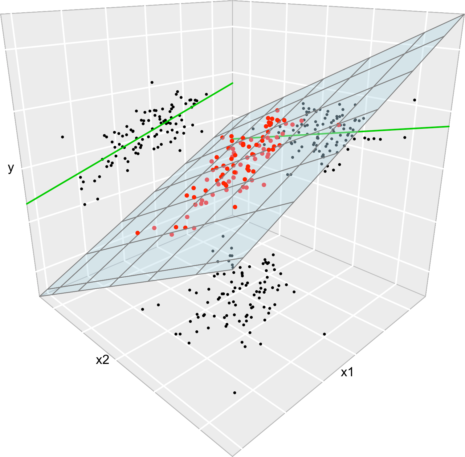
$The regression plane (blue) of $Y$ on $X_1$ and $X_2,$ and its relation with the regression lines (green lines) of $Y$ on $X_1$ (left) and of $Y$ on $X_2$ (right). The red points represent the sample for $(X_1,X_2,Y)$ and the black points the projections for $(X_1,X_2)$ (bottom), $(X_1,Y)$ (left), and $(X_2,Y)$ (right). Note that the regression plane is not a direct extension of the marginal regression lines.$

Figure B.1: The regression plane (blue) of $Y$ on $X_1$ and $X_2,$ and its relation with the regression lines (green lines) of $Y$ on $X_1$ (left) and of $Y$ on $X_2$ (right). The red points represent the sample for $(X_1,X_2,Y)$ and the black points the projections for $(X_1,X_2)$ (bottom), $(X_1,Y)$ (left), and $(X_2,Y)$ (right). Note that the regression plane is not a direct extension of the marginal regression lines.

The estimation of $\beta_0,\beta_1,\ldots,\beta_p$ is done by minimizing the so-called Residual Sum of Squares (RSS). We first need to introduce some helpful notation for this and the next section:

A sample of $(X_1,\ldots,X_p,Y)$ is denoted by $(X_{11},\ldots,X_{1p},Y_1),\ldots,$ $(X_{n1},\ldots,X_{np},Y_n),$ where $X_{ij}$ denotes the $i$ -th observation of the $j$ -th predictor $X_j.$ We denote with $\mathbf{X}_i=(X_{i1},\ldots,X_{ip})'$ to the $i$ -th observation of $(X_1,\ldots,X_p),$ so the sample is $(\mathbf{X}_{1},Y_1),\ldots,(\mathbf{X}_{n},Y_n).$
The design matrix contains all the information of the predictors and a column of ones

$\begin{align*} \mathbf{X}=\begin{pmatrix} 1 & X_{11} & \cdots & X_{1p}\\ \vdots & \vdots & \ddots & \vdots\\ 1 & X_{n1} & \cdots & X_{np} \end{pmatrix}_{n\times(p+1)}. \end{align*}$
The vector of responses $\mathbf{Y},$ the vector of coefficients $\boldsymbol\beta,$ and the vector of errors are, respectively,

$\begin{align*} \mathbf{Y}=\begin{pmatrix} Y_1 \\ \vdots \\ Y_n \end{pmatrix}_{n\times 1},\quad\boldsymbol\beta=\begin{pmatrix} \beta_0 \\ \beta_1 \\ \vdots \\ \beta_p \end{pmatrix}_{(p+1)\times 1},\text{ and } \boldsymbol\varepsilon=\begin{pmatrix} \varepsilon_1 \\ \vdots \\ \varepsilon_n \end{pmatrix}_{n\times 1}. \end{align*}$

Thanks to the matrix notation, we can turn the sample version of the multiple linear model, namely

$\begin{align*} Y_i=\beta_0 + \beta_1 X_{i1} + \ldots +\beta_p X_{ip} + \varepsilon_i,\quad i=1,\ldots,n, \end{align*}$

into something as compact as

$\begin{align*} \mathbf{Y}=\mathbf{X}\boldsymbol\beta+\boldsymbol\varepsilon. \end{align*}$

The RSS for the multiple linear regression is

$\begin{align} \text{RSS}(\boldsymbol\beta):=&\,\sum_{i=1}^n(Y_i-\beta_0-\beta_1X_{i1}-\cdots-\beta_pX_{ip})^2\nonumber\\ =&\,(\mathbf{Y}-\mathbf{X}\boldsymbol{\beta})'(\mathbf{Y}-\mathbf{X}\boldsymbol{\beta}).\tag{B.3} \end{align}$

$\text{RSS}(\boldsymbol\beta)$ aggregates the squared vertical distances from the data to a regression plane given by $\boldsymbol\beta.$ Note that the vertical distances are considered because we want to minimize the error in the prediction of $Y.$ Thus, the treatment of the variables is not symmetrical;²⁸⁸ see Figure B.2. The least squares estimators are the minimizers of (B.3):

$\begin{align*} \hat{\boldsymbol{\beta}}:=\arg\min_{\boldsymbol{\beta}\in\mathbb{R}^{p+1}} \text{RSS}(\boldsymbol{\beta}). \end{align*}$

Luckily, thanks to the matrix form of (B.3), it is simple to compute a closed-form expression for the least squares estimates:

$\begin{align} \hat{\boldsymbol{\beta}}=(\mathbf{X}'\mathbf{X})^{-1}\mathbf{X}'\mathbf{Y}.\tag{B.4} \end{align}$

Exercise B.1 $\hat{\boldsymbol{\beta}}$ can be obtained by differentiating (B.3). Prove it using that $\frac{\partial \mathbf{A}\mathbf{x}}{\partial \mathbf{x}}=\mathbf{A}$ and $\frac{\partial f(\mathbf{x})'g(\mathbf{x})}{\partial \mathbf{x}}=f(\mathbf{x})'\frac{\partial g(\mathbf{x})}{\partial \mathbf{x}}+g(\mathbf{x})'\frac{\partial f(\mathbf{x})}{\partial \mathbf{x}}$ for two vector-valued functions $f$ and $g.$

Figure B.2: The least squares regression plane $y=\hat\beta_0+\hat\beta_1x_1+\hat\beta_2x_2$ and its dependence on the kind of squared distance considered. Application available here.

Let’s check that indeed the coefficients given by R’s lm are the ones given by (B.4) in a toy linear model.

# Generates 50 points from a N(0, 1): predictors and error
set.seed(34567)
x1 <- rnorm(50)
x2 <- rnorm(50)
x3 <- x1 + rnorm(50, sd = 0.05) # Make variables dependent
eps <- rnorm(50)

# Responses
y_lin <- -0.5 + 0.5 * x1 + 0.5 * x2 + eps
y_qua <- -0.5 + x1^2 + 0.5 * x2 + eps
y_exp <- -0.5 + 0.5 * exp(x2) + x3 + eps

# Data
data_animation <- data.frame(x1 = x1, x2 = x2, y_lin = y_lin,
                             y_qua = y_qua, y_exp = y_exp)

# Call lm
# lm employs formula = response ~ predictor1 + predictor2 + ...
# (names according to the data frame names) for denoting the regression
# to be done
mod <- lm(y_lin ~ x1 + x2, data = data_animation)
summary(mod)
## 
## Call:
## lm(formula = y_lin ~ x1 + x2, data = data_animation)
## 
## Residuals:
##      Min       1Q   Median       3Q      Max 
## -2.37003 -0.54305  0.06741  0.75612  1.63829 
## 
## Coefficients:
##             Estimate Std. Error t value Pr(>|t|)    
## (Intercept)  -0.5703     0.1302  -4.380 6.59e-05 ***
## x1            0.4833     0.1264   3.824 0.000386 ***
## x2            0.3215     0.1426   2.255 0.028831 *  
## ---
## Signif. codes:  0 '***' 0.001 '**' 0.01 '*' 0.05 '.' 0.1 ' ' 1
## 
## Residual standard error: 0.9132 on 47 degrees of freedom
## Multiple R-squared:  0.276,  Adjusted R-squared:  0.2452 
## F-statistic: 8.958 on 2 and 47 DF,  p-value: 0.0005057

# mod is a list with a lot of information
# str(mod) # Long output

# Coefficients
mod$coefficients
## (Intercept)          x1          x2 
##  -0.5702694   0.4832624   0.3214894

# Application of formula (3.4)

# Matrix X
X <- cbind(1, x1, x2)

# Vector Y
Y <- y_lin

# Coefficients
beta <- solve(t(X) %*% X) %*% t(X) %*% Y
beta
##          [,1]
##    -0.5702694
## x1  0.4832624
## x2  0.3214894

Exercise B.2 Compute $\boldsymbol{\beta}$ for the regressions y_lin ~ x1 + x2, y_qua ~ x1 + x2, and y_exp ~ x2 + x3 using equation (B.4) and the function lm. Check that the fitted plane and the coefficient estimates are coherent.

Once we have the least squares estimates $\hat{\boldsymbol{\beta}},$ we can define the following two concepts:

The fitted values $\hat Y_1,\ldots,\hat Y_n,$ where

$\begin{align*} \hat Y_i:=\hat\beta_0+\hat\beta_1X_{i1}+\cdots+\hat\beta_pX_{ip},\quad i=1,\ldots,n. \end{align*}$

They are the vertical projections of $Y_1,\ldots,Y_n$ into the fitted line (see Figure B.2). In a matrix form, inputting (B.3)

$\begin{align*} \hat{\mathbf{Y}}=\mathbf{X}\hat{\boldsymbol{\beta}}=\mathbf{X}(\mathbf{X}'\mathbf{X})^{-1}\mathbf{X}'\mathbf{Y}=\mathbf{H}\mathbf{Y}, \end{align*}$

where $\mathbf{H}:=\mathbf{X}(\mathbf{X}'\mathbf{X})^{-1}\mathbf{X}'$ is called the hat matrix because it “puts the hat into $\mathbf{Y}$ ”. What it does is to project $\mathbf{Y}$ into the regression plane (see Figure B.2).
The residuals (or estimated errors) $\hat \varepsilon_1,\ldots,\hat \varepsilon_n,$ where

$\begin{align*} \hat\varepsilon_i:=Y_i-\hat Y_i,\quad i=1,\ldots,n. \end{align*}$

They are the vertical distances between actual and fitted data.

B.1.2 Model assumptions

Observe that $\hat{\boldsymbol{\beta}}$ was derived from purely geometrical arguments, not probabilistic ones. That is, we have not made any probabilistic assumption on the data generation process. However, some probabilistic assumptions are required to infer the unknown population coefficients $\boldsymbol{\beta}$ from the sample $(\mathbf{X}_1, Y_1),\ldots,(\mathbf{X}_n, Y_n).$

The assumptions of the multiple linear model are:

Linearity: $\mathbb{E}[Y|X_1=x_1,\ldots,X_p=x_p]=\beta_0+\beta_1x_1+\cdots+\beta_px_p.$
Homoscedasticity: $\mathbb{V}\text{ar}[\varepsilon_i]=\sigma^2,$ with $\sigma^2$ constant for $i=1,\ldots,n.$
Normality: $\varepsilon_i\sim\mathcal{N}(0,\sigma^2)$ for $i=1,\ldots,n.$
Independence of the errors: $\varepsilon_1,\ldots,\varepsilon_n$ are independent.

A good one-line summary of the linear model is the following (independence is assumed):

$\begin{align} Y|(X_1=x_1,\ldots,X_p=x_p)\sim \mathcal{N}(\beta_0+\beta_1x_1+\cdots+\beta_px_p,\sigma^2).\tag{B.5} \end{align}$

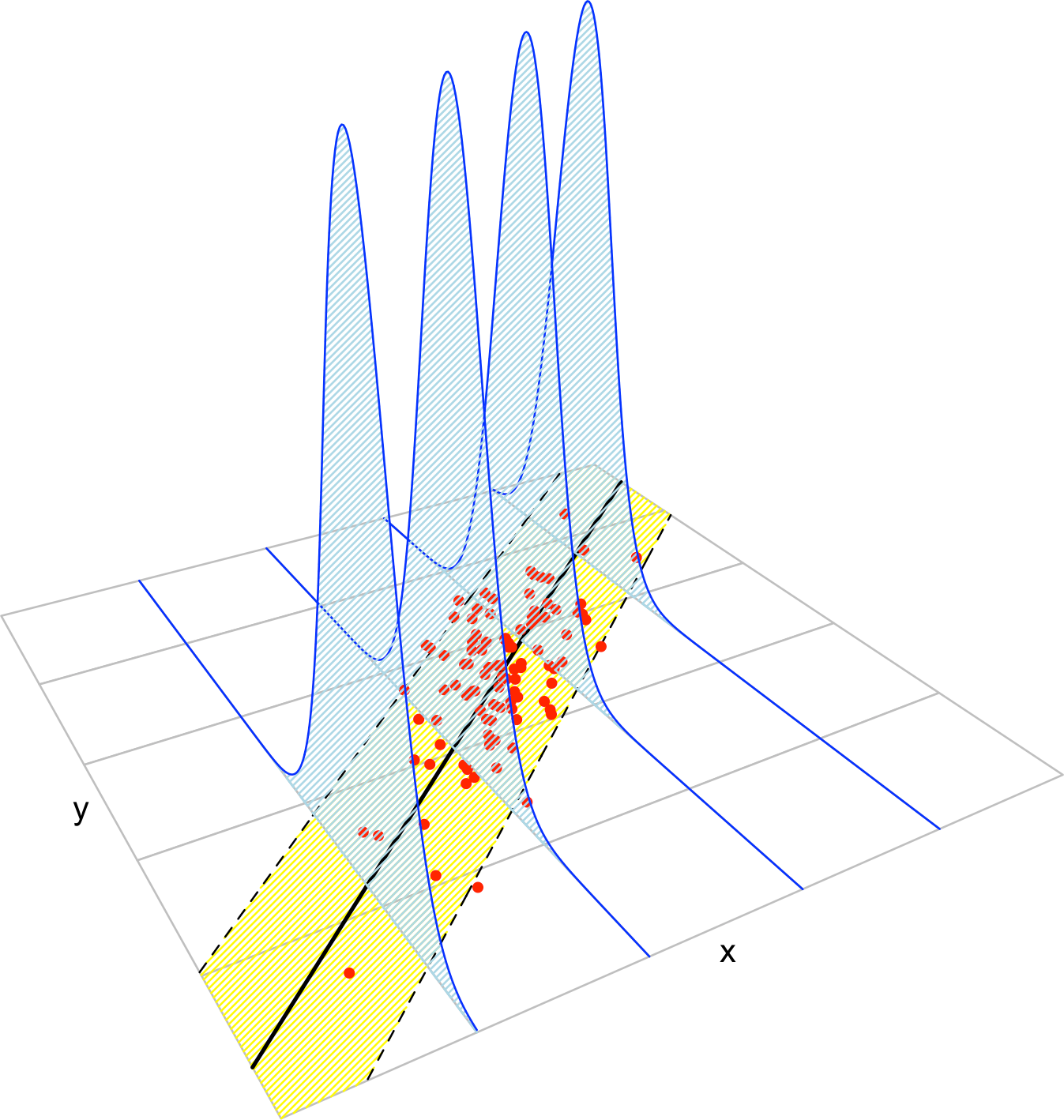
$The key concepts of the simple linear model. The blue densities denote the conditional density of $Y$ for each cut in the $X$ axis. The yellow band denotes where the $95\%$ of the data is, according to the model. The red points represent a sample following the model.$

Figure B.3: The key concepts of the simple linear model. The blue densities denote the conditional density of $Y$ for each cut in the $X$ axis. The yellow band denotes where the $95\%$ of the data is, according to the model. The red points represent a sample following the model.

Inference on the parameters $\boldsymbol\beta$ and $\sigma$ can be done, conditionally²⁸⁹ on $X_1,\ldots,X_n,$ from (B.5). We do not explore this further, referring the interested reader to, e.g., Section 2.4 in García-Portugués (2025). Instead, we remark the connection between least squares estimation and the maximum likelihood estimator derived from (B.5).

First, note that (B.5) is the population version of the linear model (it is expressed in terms of the random variables). The sample version that summarizes assumptions i–iv is

$\begin{align*} \mathbf{Y}|\mathbf{X}\sim \mathcal{N}_n(\mathbf{X}\boldsymbol{\beta},\sigma^2\mathbf{I}_n). \end{align*}$

Using this result, it is easy to obtain the log-likelihood function of $Y_1,\ldots,Y_n$ conditionally on $\mathbf{X}_1,\ldots,\mathbf{X}_n$ as²⁹⁰

$\begin{align} \ell(\boldsymbol{\beta})=\log\phi_{\sigma^2\mathbf{I}_n}(\mathbf{Y}-\mathbf{X}\boldsymbol{\beta})=\sum_{i=1}^n\log\phi_{\sigma}(Y_i-(\mathbf{X}\boldsymbol{\beta})_i).\tag{B.6} \end{align}$

Finally, the following result justifies the consideration of the least squares estimate: it equals the maximum likelihood estimator derived under assumptions i–iv.

Theorem B.1 Under assumptions i–iv, the maximum likelihood estimator of $\boldsymbol{\beta}$ is the least squares estimate (B.4):

$\begin{align*} \hat{\boldsymbol{\beta}}_\mathrm{ML}=\arg\max_{\boldsymbol{\beta}\in\mathbb{R}^{p+1}}\ell(\boldsymbol{\beta})=(\mathbf{X}'\mathbf{X})^{-1}\mathbf{X}'\mathbf{Y}. \end{align*}$

Proof. Expanding the first equality at (B.6) gives²⁹¹

$\begin{align*} \ell(\boldsymbol{\beta})=-\log((2\pi)^{n/2}\sigma^n)-\frac{1}{2\sigma^2}(\mathbf{Y}-\mathbf{X}\boldsymbol{\beta})'(\mathbf{Y}-\mathbf{X}\boldsymbol{\beta}). \end{align*}$

Optimizing $\ell$ does not require knowledge on $\sigma^2,$ since differentiating with respect to $\boldsymbol{\beta}$ and equating to zero gives (see Exercise B.1) $\frac{1}{\sigma^2}(\mathbf{Y}-\mathbf{X}\boldsymbol{\beta})'\mathbf{X}=\mathbf{0}.$ Solving the equation gives the form for $\hat{\boldsymbol{\beta}}_\mathrm{ML}.$

Exercise B.3 Conclude the proof of Theorem B.1.

References

García-Portugués, E. 2025. Notes for Predictive Modeling. https://bookdown.org/egarpor/PM-UC3M/.

Not to confuse with a sample!↩︎
If that were the case, we would consider perpendicular distances, which yield Principal Component Analysis (PCA).↩︎
We assume that the randomness is on the response only.↩︎
Recall that $\phi_{\boldsymbol{\Sigma}}(\cdot-\boldsymbol{\mu})$ and $\phi_{\sigma}(\cdot-\mu)$ denote the pdf of a $\mathcal{N}_p(\boldsymbol{\mu},\boldsymbol{\Sigma})$ and a $\mathcal{N}(\mu,\sigma^2),$ respectively.↩︎
Since $|\sigma^2\mathbf{I}_n|^{1/2}=\sigma^{n}.$ ↩︎