B.2 Logistic regression

B.2.1 Model formulation

When the response $Y$ can take two values only, codified for convenience as $1$ (success) and $0$ (failure), $Y$ is called a binary variable. A binary variable, known also as a Bernoulli variable, is a $\mathrm{B}(1, p).$²⁹²

If $Y$ is a binary variable and $X_1,\ldots,X_p$ are predictors associated with $Y,$ the purpose in logistic regression is to estimate

$$\begin{align} p(x_1,\ldots,x_p):=&\,\mathbb{P}[Y=1|X_1=x_1,\ldots,X_p=x_p]\nonumber\\ =&\,\mathbb{E}[Y|X_1=x_1,\ldots,X_p=x_p],\tag{B.7} \end{align}$$

this is, how the probability of $Y=1$ is changing according to particular values, denoted by $x_1,\ldots,x_p,$ of the predictors $X_1,\ldots,X_p.$ A tempting possibility is to consider a linear model for (B.7), $p(x_1,\ldots,x_p)=\beta_0+\beta_1x_1+\cdots+\beta_px_p.$ However, such a model will run into serious problems inevitably: negative probabilities and probabilities greater than one will arise.

A solution is to consider a function to encapsulate the value of $z=\beta_0+\beta_1x_1+\cdots+\beta_px_p,$ in $\mathbb{R},$ and map it back to $[0,1].$ There are several alternatives to do so, based on distribution functions $F:\mathbb{R}\longrightarrow[0,1]$ that deliver $y=F(z)\in[0,1].$ Different choices of $F$ give rise to different models, the most common one being the logistic distribution function:

$$\begin{align*} \mathrm{logistic}(z):=\frac{e^z}{1+e^z}=\frac{1}{1+e^{-z}}. \end{align*}$$

Its inverse, $F^{-1}:[0,1]\longrightarrow\mathbb{R},$ known as the logit function, is

$$\begin{align*} \mathrm{logit}(p):=\mathrm{logistic}^{-1}(p)=\log\frac{p}{1-p}. \end{align*}$$

This is a link function, that is, a function that maps a given space (in this case $[0,1]$) onto $\mathbb{R}.$ The term link function is used in generalized linear models, which follow exactly the same philosophy of the logistic regression – mapping the domain of $Y$ to $\mathbb{R}$ in order to apply there a linear model. As said above, different link functions are possible, but we will concentrate here exclusively on the logit as a link function.

The logistic model is defined as the next parametric form for (B.7):

$$\begin{align} p(x_1,\ldots,x_p)&=\mathrm{logistic}(\beta_0+\beta_1x_1+\cdots+\beta_px_p)\nonumber\\ &=\frac{1}{1+e^{-(\beta_0+\beta_1x_1+\cdots+\beta_px_p)}}.\tag{B.8} \end{align}$$

The linear form inside the exponent has a clear interpretation:

• If $\beta_0+\beta_1x_1+\cdots+\beta_px_p=0,$ then $p(x_1,\ldots,x_p)=\frac{1}{2}$ ($Y=1$ and $Y=0$ are equally likely).
• If $\beta_0+\beta_1x_1+\cdots+\beta_px_p<0,$ then $p(x_1,\ldots,x_p)<\frac{1}{2}$ ($Y=1$ less likely).
• If $\beta_0+\beta_1x_1+\cdots+\beta_px_p>0,$ then $p(x_1,\ldots,x_p)>\frac{1}{2}$ ($Y=1$ more likely).

To be more precise on the interpretation of the coefficients $\beta_0,\ldots,\beta_p$ we need to introduce the concept of odds. The odds is an equivalent form of expressing the distribution of probabilities in a binary variable. Since $\mathbb{P}[Y=1]=p$ and $\mathbb{P}[Y=0]=1-p,$ both the success and failure probabilities can be inferred from $p.$ Instead of using $p$ to characterize the distribution of $Y,$ we can use

$$\begin{align} \mathrm{odds}(Y)=\frac{p}{1-p}=\frac{\mathbb{P}[Y=1]}{\mathbb{P}[Y=0]}.\tag{B.9} \end{align}$$

The odds is the ratio between the probability of success and the probability of failure. It is extensively used in betting due to its better interpretability.²⁹³ Conversely, if the odds of $Y$ is given, we can easily know what is the probability of success $p,$ using the inverse²⁹⁴ of (B.9):

$$\begin{align*} p=\mathbb{P}[Y=1]=\frac{\text{odds}(Y)}{1+\text{odds}(Y)}. \end{align*}$$

Remark. Recall that the odds is a number in $[0,+\infty].$ The $0$ and $+\infty$ values are attained for $p=0$ and $p=1,$ respectively. The log-odds (or logit) is a number in $[-\infty,+\infty].$

We can rewrite (B.8) in terms of the odds (B.9). If we do so, then

$$\begin{align*} \mathrm{odds}(Y|&X_1=x_1,\ldots,X_p=x_p)\\ &=\frac{p(x_1,\ldots,x_p)}{1-p(x_1,\ldots,x_p)}\\ &=e^{\beta_0+\beta_1x_1+\cdots+\beta_px_p}\\ &=e^{\beta_0}e^{\beta_1x_1}\cdots e^{\beta_px_p}. \end{align*}$$

This provides the following interpretation of the coefficients:

• $e^{\beta_0}$: is the odds of $Y=1$ when $X_1=\cdots=X_p=0.$
• $e^{\beta_j},$ $1\leq j\leq k$: is the multiplicative increment of the odds for an increment of one unit in $X_j=x_j,$ provided that the remaining variables do not change. If the increment in $X_j$ is of $r$ units, then the multiplicative increment in the odds is $(e^{\beta_j})^r.$

B.2.2 Model assumptions and estimation

Some probabilistic assumptions are required to perform inference on the model parameters $\boldsymbol\beta$ from a sample $(\mathbf{X}_1, Y_1),\ldots,(\mathbf{X}_n, Y_n).$ These assumptions are somehow simpler than the ones for linear regression.

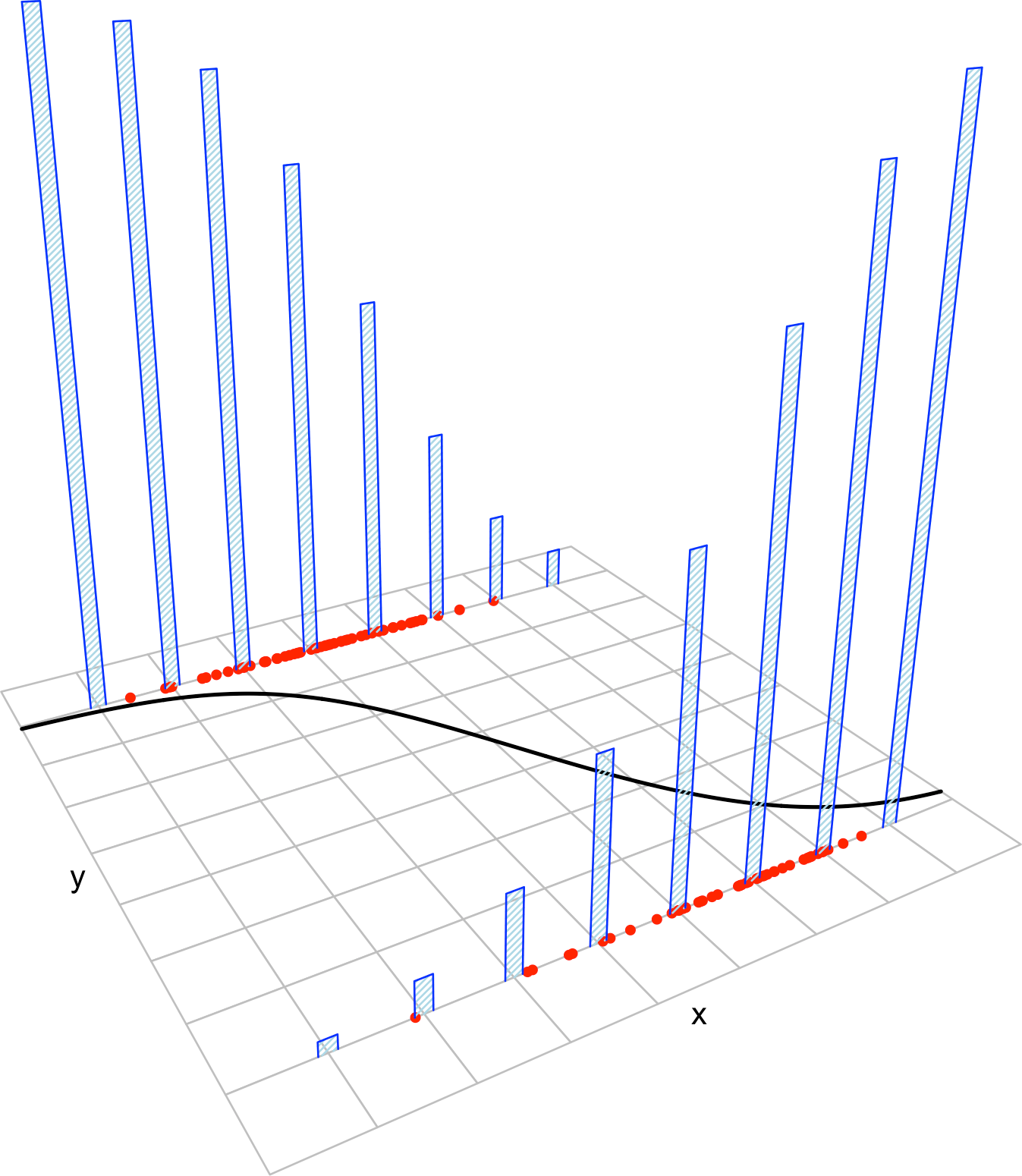
Figure B.4: The key concepts of the logistic model. The blue bars represent the conditional distribution of probability of $Y$ for each cut in the $X$ axis. The red points represent a sample following the model.

The assumptions of the logistic model are the following:

1. Linearity in the logit:²⁹⁵ $\mathrm{logit}(p(\mathbf{x}))=\log\frac{ p(\mathbf{x})}{1-p(\mathbf{x})}=\beta_0+\beta_1x_1+\cdots+\beta_px_p.$
2. Binariness: $Y_1,\ldots,Y_n$ are binary variables.
3. Independence: $Y_1,\ldots,Y_n$ are independent.

A good one-line summary of the logistic model is the following (independence is assumed):

$$\begin{align*} Y|(X_1=x_1,\ldots,X_p=x_p)&\sim\mathrm{Ber}\left(\mathrm{logistic}(\beta_0+\beta_1x_1+\cdots+\beta_px_p)\right)\\ &=\mathrm{Ber}\left(\frac{1}{1+e^{-(\beta_0+\beta_1x_1+\cdots+\beta_px_p)}}\right). \end{align*}$$

Since $Y_i\sim \mathrm{Ber}(p(\mathbf{X}_i)),$ $i=1,\ldots,n,$ the log-likelihood of $\boldsymbol{\beta}$ is

$$\begin{align} \ell(\boldsymbol{\beta})=&\,\sum_{i=1}^n\log\left(p(\mathbf{X}_i)^{Y_i}(1-p(\mathbf{X}_i))^{1-Y_i}\right)\nonumber\\ =&\,\sum_{i=1}^n\left\{Y_i\log(p(\mathbf{X}_i))+(1-Y_i)\log(1-p(\mathbf{X}_i))\right\}.\tag{B.10} \end{align}$$

Unfortunately, due to the nonlinearity of the optimization problem, there are no explicit solutions for $\hat{\boldsymbol{\beta}}.$ These have to be obtained numerically by means of an iterative procedure, which may run into problems in low-sample situations with perfect classification. Unlike in the linear model, inference is not exact from the assumptions, but rather approximate in terms of maximum likelihood theory. We do not explore this further and refer the interested reader to, e.g., Section 5.3 in García-Portugués (2025).

Figure B.5: The logistic regression fit and its dependence on $\beta_0$ (horizontal displacement) and $\beta_1$ (steepness of the curve). Recall the effect of the sign of $\beta_1$ on the curve: if positive, the logistic curve has an “s” form; if negative, the form is a reflected “s”. Application available here.

Figure B.5 shows how the log-likelihood changes with respect to the values for $(\beta_0,\beta_1)$ in three data patterns. The data of the illustration has been generated with the following code.

# Data
set.seed(34567)
x <- rnorm(50, sd = 1.5)
y1 <- -0.5 + 3 * x
y2 <- 0.5 - 2 * x
y3 <- -2 + 5 * x
y1 <- rbinom(50, size = 1, prob = 1 / (1 + exp(-y1)))
y2 <- rbinom(50, size = 1, prob = 1 / (1 + exp(-y2)))
y3 <- rbinom(50, size = 1, prob = 1 / (1 + exp(-y3)))

# Data
data_mle <- data.frame(x = x, y1 = y1, y2 = y2, y3 = y3)

Let’s check that indeed the coefficients given by R’s glm are the ones that maximize the likelihood of the animation of Figure B.5. We do so for y ~ x1.

# Call glm
# glm employs formula = response ~ predictor1 + predictor2 + ...
# (names according to the data frame names) for denoting the regression
# to be done. We need to specify family = "binomial" to make a
# logistic regression
mod <- glm(y1 ~ x, family = "binomial", data = data_mle)
summary(mod)
## 
## Call:
## glm(formula = y1 ~ x, family = "binomial", data = data_mle)
## 
## Deviance Residuals: 
##      Min        1Q    Median        3Q       Max  
## -2.47853  -0.40139   0.02097   0.38880   2.12362  
## 
## Coefficients:
##             Estimate Std. Error z value Pr(>|z|)    
## (Intercept)  -0.1692     0.4725  -0.358 0.720274    
## x             2.4282     0.6599   3.679 0.000234 ***
## ---
## Signif. codes:  0 '***' 0.001 '**' 0.01 '*' 0.05 '.' 0.1 ' ' 1
## 
## (Dispersion parameter for binomial family taken to be 1)
## 
##     Null deviance: 69.315  on 49  degrees of freedom
## Residual deviance: 29.588  on 48  degrees of freedom
## AIC: 33.588
## 
## Number of Fisher Scoring iterations: 6

# mod is a list with a lot of information
# str(mod) # Long output

# Coefficients
mod$coefficients
## (Intercept)           x 
##  -0.1691947   2.4281626

# Plot the fitted regression curve
x_grid <- seq(-5, 5, l = 200)
y_grid <- 1 / (1 + exp(-(mod$coefficients[1] + mod$coefficients[2] * x_grid)))
plot(x_grid, y_grid, type = "l", col = 2, xlab = "x", ylab = "y")
points(x, y1)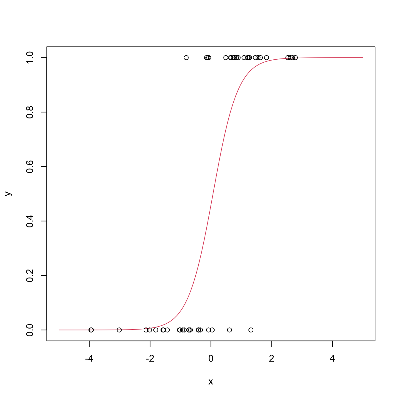

Exercise B.4 For the regressions y ~ x2 and y ~ x3, do the following:

1. Check that $\boldsymbol{\beta}$ is indeed maximizing the likelihood as compared with Figure B.5.
2. Plot the fitted logistic curve and compare it with the one in Figure B.5.

References

García-Portugués, E. 2025. Notes for Predictive Modeling. https://bookdown.org/egarpor/PM-UC3M/.

---

292. Recall that $\mathbb{E}[\mathrm{B}(1, p)]=\mathbb{P}[\mathrm{B}(1, p)=1]=p.$↩︎

293. For example, if a horse $Y$ has a probability $p=2/3$ of winning a race ($Y=1$), then the odds of the horse is $\text{odds}=\frac{p}{1-p}=\frac{2/3}{1/3}=2.$ This means that the horse has a probability of winning that is twice larger than the probability of losing. This is sometimes written as a $2:1$ or $2 \times 1$ (spelled “two-to-one”).↩︎

294. For example, if the odds of the horse was $5,$ that would correspond to a probability of winning $p=5/6.$↩︎

295. An equivalent way of stating this assumption is $p(\mathbf{x})=\mathrm{logistic}(\beta_0+\beta_1x_1+\cdots+\beta_px_p).$↩︎