Chapter 2 Kernel density estimation I

A random variable \(X\) is completely characterized by its cdf. Hence, an estimation of the cdf yields estimates for different characteristics of \(X\) as side-products by plugging, in these characteristics, the ecdf \(F_n\) instead of the \(F.\) For example¹¹, the mean \(\mu=\mathbb{E}[X]=\int x\,\mathrm{d}F(x)\) can be estimated by \(\int x \,\mathrm{d}F_n(x)=\frac{1}{n}\sum_{i=1}^n X_i=\bar X.\)

Despite their usefulness and many advantages, cdfs are hard to visualize and interpret, a consequence of their cumulative-based definition.

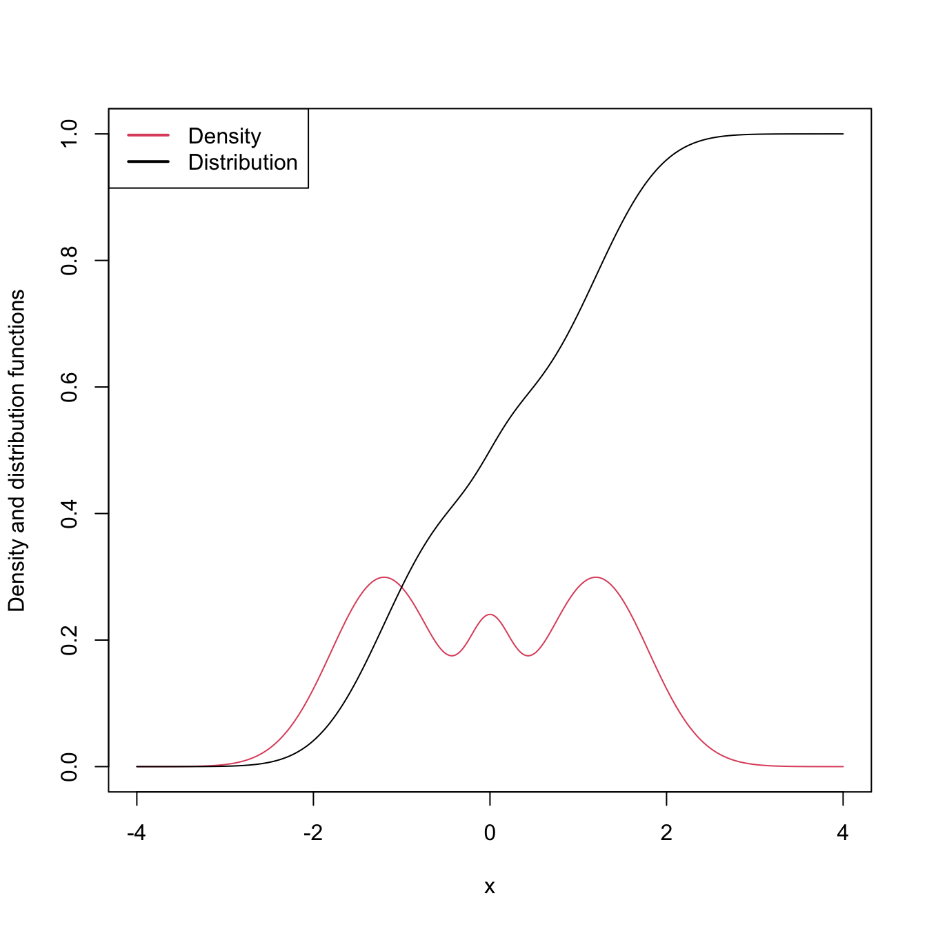
Figure 2.1: The pdf and cdf of a mixture of three normals. The pdf yields better insights into the structure of the continuous random variable \(X\) than the cdf does.

Densities, on the other hand, are easy to visualize and interpret, making them ideal tools for data exploration of continuous random variables. They provide immediate graphical information about the highest-density regions, modes, and shape of the support of \(X.\) In addition, densities also completely characterize continuous random variables. Yet, even though a pdf follows from a cdf by the relation \(f=F',\) density estimation does not follow immediately from the ecdf \(F_n,\) since this function is not differentiable¹². Hence the need for specific procedures for estimating \(f\) that we will see in this chapter.

---

11. Another example is the \(p\)-quantile \(x_p:=F^{(-1)}(p),\) where \(F^{(-1)}(u):=\inf\{x\in\mathbb{R}:F(x)\geq u\}\) is the pseudo-inverse of the cdf \(F.\) Then, \(x_p\) can be estimated by the sample \(p\)-quantile \(\hat{x}_p:=F_n^{(-1)}(p).\)↩︎

12. Is not even continuous!↩︎