A Confidence intervals for the density function
Obtaining a Confidence Interval (CI) for \(f(x)\) is a challenging task. Thanks to the bias results286 seen in Section 2.3, we know that the kde is biased for finite sample sizes and it is only asymptotically unbiased when \(h\to0.\) This bias is called the smoothing bias and, in essence, complicates the obtention of CIs for \(f(x),\) but not for \((K_h*f)(x).\) Let’s see the differences between these two objects with an illustrative example.
Some well-known facts for normal densities (see Appendix C in Wand and Jones (1995)) are:
\[\begin{align} (\phi_{\sigma_1}(\cdot-\mu_1)*\phi_{\sigma_2}(\cdot-\mu_2))(x)&=\phi_{(\sigma_1^2+\sigma_2^2)^{1/2}}(x-\mu_1-\mu_2),\tag{A.1}\\ \int\phi_{\sigma_1}(x-\mu_1)\phi_{\sigma_2}(x-\mu_2)\,\mathrm{d}x&=\phi_{(\sigma_1^2+\sigma_2^2)^{1/2}}(\mu_1-\mu_2),\\ \phi_{\sigma}(x-\mu)^r&=\frac{1}{\sigma^{r-1}}(2\pi)^{(1-r)/2}\phi_{\sigma/ r^{1/2}}(x-\mu)\frac{1}{r^{1/2}}.\tag{A.2} \end{align}\]
Consequently, if \(K=\phi\) (i.e., \(K_h=\phi_h\)) and \(f(\cdot)=\phi_\sigma(\cdot-\mu)\):
\[\begin{align} (K_h*f)(x)&=\phi_{(h^2+\sigma^2)^{1/2}}(x-\mu),\tag{A.3}\\ (K_h^2*f)(x)&=\left(\frac{1}{(2\pi)^{1/2}h}\phi_{h/2^{1/2}}/2^{1/2}*f\right)(x)\nonumber\\ &=\frac{1}{2\pi^{1/2}h}\left(\phi_{h/2^{1/2}}*f\right)(x)\nonumber\\ &=\frac{1}{2\pi^{1/2}h}\phi_{(h^2/2+\sigma^2)^{1/2}}(x-\mu).\tag{A.4} \end{align}\]
Thus, the exact expectation of the kde for estimating the density of a \(\mathcal{N}(\mu,\sigma^2)\) is precisely the density of a \(\mathcal{N}(\mu,\sigma^2+h^2).\) Clearly, when \(h\to0,\) we can see how the bias disappears. Removing this finite-sample size bias is not simple: if the bias is expanded, \(f''\) appears. Hence, to attempt to unbias \(\hat{f}(\cdot;h)\) we have to estimate \(f'',\) which is a harder task than estimating \(f.\) As seen in Section 3.2, taking second derivatives on the kde does not work out-of-the-box, since the bandwidths for estimating \(f\) and \(f''\) scale differently.
The previous deadlock can be solved if we limit our ambitions. Rather than constructing a confidence interval for \(f(x),\) we can construct it for \(\mathbb{E}[\hat{f}(x;h)]=(K_h*f)(x).\) There is nothing wrong with this change of view, as long as we are explicitly report the CI as that for \((K_h*f)(x)\) and not for \(f(x).\)
The building block for the CI for \(\mathbb{E}[\hat{f}(x;h)]=(K_h*f)(x)\) is the first result287 in Theorem 2.2, which concludes that
\[\begin{align*} \sqrt{nh}(\hat{f}(x;h)-\mathbb{E}[\hat{f}(x;h)])\stackrel{d}{\longrightarrow}\mathcal{N}(0,R(K)f(x)). \end{align*}\]
Plugging \(\hat{f}(x;h)=f(x)+O_\mathbb{P}\big(h^2+(nh)^{-1/2}\big)=f(x)(1+o_\mathbb{P}(1))\) (see Exercise 2.10) as an estimate for \(f(x)\) in the variance, we have by the Slutsky’s theorem that
\[\begin{align*} \sqrt{\frac{nh}{R(K)\hat{f}(x;h)}}&(\hat{f}(x;h)-\mathbb{E}[\hat{f}(x;h)])\\ &=\sqrt{\frac{nh}{R(K)f(x)}}(\hat{f}(x;h)-\mathbb{E}[\hat{f}(x;h)])(1+o_\mathbb{P}(1))\\ &\stackrel{d}{\longrightarrow}\mathcal{N}(0,1). \end{align*}\]
Therefore, an asymptotic \(100(1-\alpha)\%\) confidence interval for \(\mathbb{E}[\hat{f}(x;h)]\) that can be straightforwardly computed is
\[\begin{align} I=\left(\hat{f}(x;h)\pm z_{\alpha/2}\sqrt{\frac{R(K)\hat{f}(x;h)}{nh}}\right).\tag{A.5} \end{align}\]
Remark. Several points regarding (A.5) require proper awareness:
- As announced, the CI is meant for \(\mathbb{E}[\hat{f}(x;h)]=(K_h*f)(x),\) not \(f(x),\) as it does not account for the smoothing bias.
- This is a pointwise CI: \(\mathbb{P}\left[\mathbb{E}[\hat{f}(x;h)]\in I\right]\approx 1-\alpha\) for each \(x\in\mathbb{R}.\) That is, \(\mathbb{P}\left[\mathbb{E}[\hat{f}(x;h)]\in I,\,\forall x\in\mathbb{R}\right]\neq 1-\alpha.\)
- The CI relies on an approximation of \(f(x)\) in the variance, done by \(\hat{f}(x;h)=f(x)+O_\mathbb{P}\big(h^2+(nh)^{-1/2}\big).\) Additionally, the convergence to a normal distribution happens at rate \(\sqrt{nh}.\) Hence, both \(h\) and \(nh\) need to be small and large, respectively, for a good coverage.
- The CI is built using a deterministic bandwidth \(h\) (i.e., not data-driven), which is not usually the case in practice. If a bandwidth selector is employed, the coverage may be affected, especially for small \(n.\)
We illustrate the construction of the CI in (A.5) for the situation where the reference density is a \(\mathcal{N}(\mu,\sigma^2)\) and the normal kernel is employed. This allows using (A.3) and (A.4), in combination with (2.11) and (2.12), to obtain
\[\begin{align*} \mathbb{E}[\hat{f}(x;h)]&=\phi_{(h^2+\sigma^2)^{1/2}}(x-\mu),\\ \mathbb{V}\mathrm{ar}[\hat{f}(x;h)]&=\frac{1}{n}\left(\frac{\phi_{(h^2/2+\sigma^2)^{1/2}}(x-\mu)}{2\pi^{1/2}h}-(\phi_{(h^2+\sigma^2)^{1/2}}(x-\mu))^2\right). \end{align*}\]
These exact results are useful to benchmark (A.5) with the asymptotic CI that employs the exact variance of \(\hat{f}(x;h)\):
\[\begin{align} \left(\hat{f}(x;h)\pm z_{\alpha/2} \sqrt{\mathbb{V}\mathrm{ar}[\hat{f}(x;h)]}\right).\tag{A.6} \end{align}\]
The following chunk of code evaluates the proportion of times that \(\mathbb{E}[\hat{f}(x;h)]\) belongs to \(I\) for each \(x\in\mathbb{R},\) both with estimated or known variance in the asymptotic distribution.
# R(K) for a normal
Rk <- 1 / (2 * sqrt(pi))

# Generate a sample from a N(mu, sigma^2)
n <- 100
mu <- 0
sigma <- 1
set.seed(123456)
x <- rnorm(n = n, mean = mu, sd = sigma)

# Compute the kde (NR bandwidth)
kde <- density(x = x, from = -4, to = 4, n = 1024, bw = "nrd")

# Selected bandwidth
h <- kde$bw

# Estimate the variance
var_kde_hat <- kde$y * Rk / (n * h)

# True expectation and variance (because the density is a normal)
E_kde <- dnorm(x = kde$x, mean = mu, sd = sqrt(sigma^2 + h^2))
var_kde <- (dnorm(kde$x, mean = mu, sd = sqrt(h^2 / 2 + sigma^2)) /
              (2 * sqrt(pi) * h) - E_kde^2) / n

# CI with estimated variance
alpha <- 0.05
z_alpha2 <- qnorm(1 - alpha / 2)
ci_low_1 <- kde$y - z_alpha2 * sqrt(var_kde_hat)
ci_up_1 <- kde$y + z_alpha2 * sqrt(var_kde_hat)

# CI with known variance
ci_low_2 <- kde$y - z_alpha2 * sqrt(var_kde)
ci_up_2 <- kde$y + z_alpha2 * sqrt(var_kde)

# Plot estimate, CIs and expectation
plot(kde, main = "Density and CIs", ylim = c(0, 1))
lines(kde$x, ci_low_1, col = "gray")
lines(kde$x, ci_up_1, col = "gray")
lines(kde$x, ci_low_2, col = "gray", lty = 2)
lines(kde$x, ci_up_2, col = "gray", lty = 2)
lines(kde$x, E_kde, col = "red")
legend("topright", legend = c("Estimate", "CI estimated var",
                              "CI known var", "Smoothed density"),
       col = c("black", "gray", "gray", "red"), lwd = 2, lty = c(1, 1, 2, 1))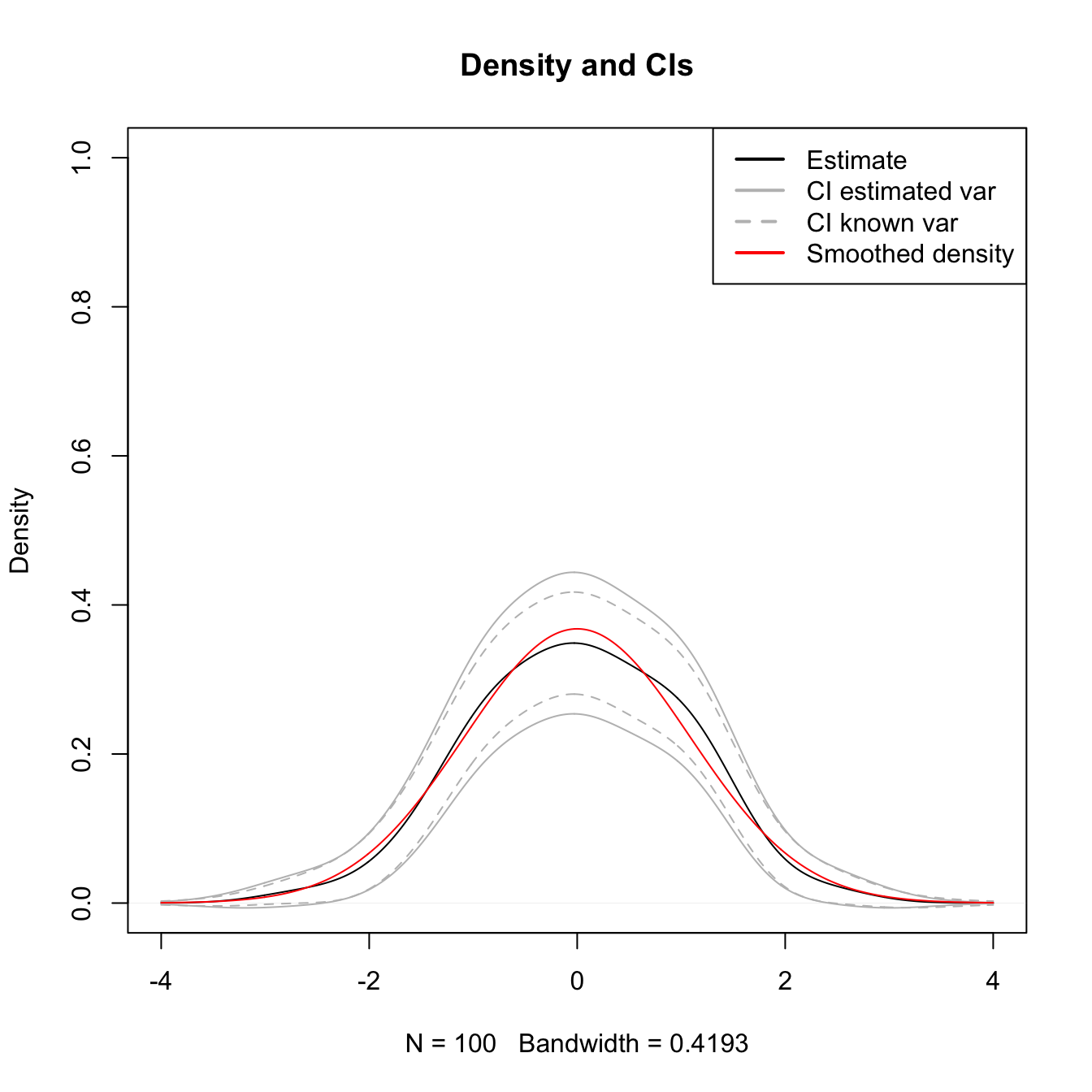
Figure A.1: The CIs (A.5) and (A.6) for \(\mathbb{E}\lbrack\hat{f}(x;h)\rbrack\) with estimated and known variances.
The above experiment shows the CI, but it does not give any insight into the effective coverage of the CI. The following simulation exercise precisely addresses this issue. As seen from Figure A.2, the estimation of the kde’s variance has a considerable impact on the coverage of the CI in the low-density regions, and it is reasonably fine for the higher density regions.
# Simulation setting
n <- 200; h <- 0.15
mu <- 0; sigma <- 1 # Normal parameters
M <- 5e2 # Number of replications in the simulation
n_grid <- 512 # Number of x's for computing the kde
alpha <- 0.05; z_alpha2 <- qnorm(1 - alpha / 2) # alpha for CI

# Compute expectation and variance
kde <- density(x = 0, bw = h, from = -4, to = 4, n = n_grid) # Just for kde$x
E_kde <- dnorm(x = kde$x, mean = mu, sd = sqrt(sigma^2 + h^2))
var_kde <- (dnorm(kde$x, mean = mu, sd = sqrt(h^2 / 2 + sigma^2)) /
              (2 * sqrt(pi) * h) - E_kde^2) / n

# For storing if the mean is inside the CI
inside_ci_1 <- inside_ci_2 <- matrix(nrow = M, ncol = n_grid)

# Simulation
set.seed(12345)
for (i in 1:M) {

  # Sample & kde
  x <- rnorm(n = n, mean = mu, sd = sigma)
  kde <- density(x = x, bw = h, from = -4, to = 4, n = n_grid)
  sd_kde_hat <- sqrt(kde$y * Rk / (n * h))

  # CI with estimated variance
  ci_low_1 <- kde$y - z_alpha2 * sd_kde_hat
  ci_up_1 <- kde$y + z_alpha2 * sd_kde_hat

  # CI with known variance
  ci_low_2 <- kde$y - z_alpha2 * sqrt(var_kde)
  ci_up_2 <- kde$y + z_alpha2 * sqrt(var_kde)

  # Check if for each x the mean is inside the CI
  inside_ci_1[i, ] <- E_kde > ci_low_1 & E_kde < ci_up_1
  inside_ci_2[i, ] <- E_kde > ci_low_2 & E_kde < ci_up_2

}

# Plot results
plot(kde$x, colMeans(inside_ci_1), ylim = c(0.25, 1), type = "l",
     main = "Empirical coverage of CIs", xlab = "x", ylab = "Coverage")
lines(kde$x, colMeans(inside_ci_2), col = 4)
abline(h = 1 - alpha, col = 2)
abline(h = 1 - alpha + c(-1, 1) * qnorm(0.975) *
         sqrt(alpha * (1 - alpha) / M), col = 2, lty = 2)
legend(x = "bottom", legend = c("CI estimated var", "CI known var",
                                "Nominal level",
                                "95% CI for the nominal level"),
       col = c(1, 4, 2, 2), lwd = 2, lty = c(1, 1, 1, 2))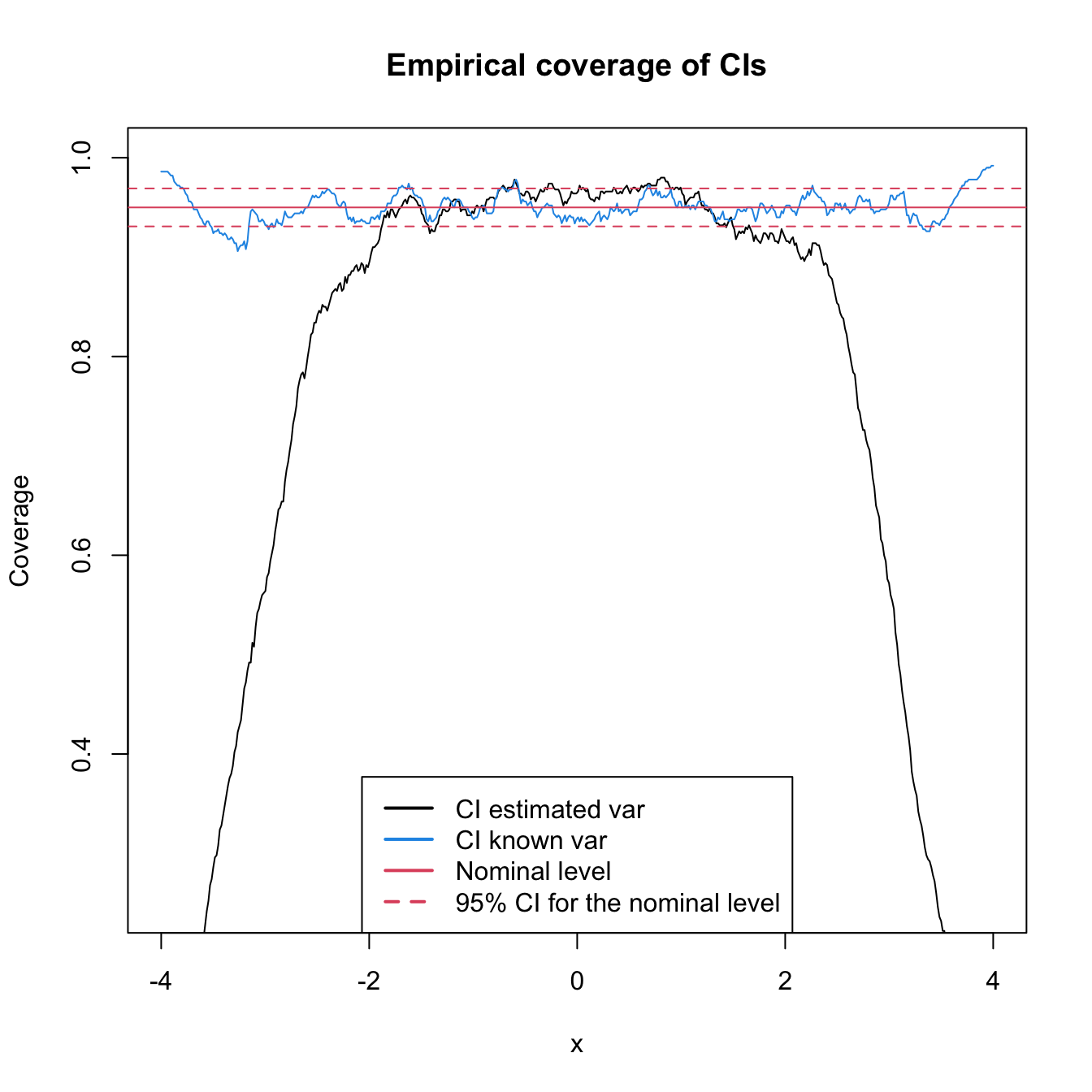
Figure A.2: Empirical coverage of the CIs (A.5) and (A.6) for \(\mathbb{E}\lbrack\hat{f}(x;h)\rbrack\) with estimated and known variances.
Exercise A.1 Explore the coverage of the asymptotic CI for varying values of \(h.\) To that end, adapt the previous code to work in a manipulate environment like the example given below.
# Sample
x <- rnorm(100)

# Simple plot of kde for varying h
manipulate::manipulate({

  kde <- density(x = x, from = -4, to = 4, bw = h)
  plot(kde, ylim = c(0, 1), type = "l", main = "")
  curve(dnorm(x), from = -4, to = 4, col = 2, add = TRUE)
  rug(x)

}, h = manipulate::slider(min = 0.01, max = 2, initial = 0.5, step = 0.01))
Exercise A.2 (Exercise 6.9.5 in Wasserman (2006)) Data on the salaries of the chief executive officer of \(60\) companies is available at http://lib.stat.cmu.edu/DASL/Datafiles/ceodat.html (alternative link). Investigate the distribution of salaries using a kde. Use \(\hat{h}_\mathrm{LSCV}\) to choose the amount of smoothing. Also, consider \(\hat{h}_\mathrm{RT}.\) There appear to be a few bumps in the density. Are they real? Use confidence bands to address this question. Finally, comment on the resulting estimates.