1.1 Probability review
1.1.1 Random variables
A triple \((\Omega,\mathcal{A},\mathbb{P})\) is called a probability space. \(\Omega\) represents the sample space, the set of all possible individual outcomes of a random experiment. \(\mathcal{A}\) is a \(\sigma\)-field, a class of subsets of \(\Omega\) that is closed under complementation and numerable unions, and such that \(\Omega\in\mathcal{A}.\) \(\mathcal{A}\) represents the collection of possible events (combinations of individual outcomes) that are assigned a probability by the probability measure \(\mathbb{P}.\) A random variable is a map \(X:\Omega\longrightarrow\mathbb{R}\) such that \(X^{-1}((-\infty,x])=\{\omega\in\Omega:X(\omega)\leq x\}\in\mathcal{A},\) \(\forall x\in\mathbb{R}\) (the set \(X^{-1}((-\infty,x])\) of possible outcomes of \(X\) is said measurable).
1.1.2 Cumulative distribution and probability density functions
The cumulative distribution function (cdf) of a random variable \(X\) is \(F(x):=\mathbb{P}[X\leq x].\) When an independent and identically distributed (iid) sample \(X_1,\ldots,X_n\) is given, the cdf can be estimated by the empirical distribution function (ecdf)
\[\begin{align} F_n(x)=\frac{1}{n}\sum_{i=1}^n1_{\{X_i\leq x\}}, \tag{1.1} \end{align}\]
where \(1_A:=\begin{cases}1,&A\text{ is true},\\0,&A\text{ is false}\end{cases}\) is an indicator function.2
Continuous random variables are characterized by either the cdf \(F\) or the probability density function (pdf) \(f=F',\) the latter representing the infinitesimal relative probability of \(X\) per unit of length. We write \(X\sim F\) (or \(X\sim f\)) to denote that \(X\) has a cdf \(F\) (or a pdf \(f\)). If two random variables \(X\) and \(Y\) have the same distribution, we write \(X\stackrel{d}{=}Y.\)
1.1.3 Expectation
The expectation operator is constructed using the Riemann–Stieltjes “\(\,\mathrm{d}F(x)\)” integral.3 Hence, for \(X\sim F,\) the expectation of \(g(X)\) is
\[\begin{align*} \mathbb{E}[g(X)]:=&\,\int g(x)\,\mathrm{d}F(x)\\ =&\, \begin{cases} \displaystyle\int g(x)f(x)\,\mathrm{d}x,&\text{ if }X\text{ is continuous,}\\\displaystyle\sum_{\{x\in\mathbb{R}:\mathbb{P}[X=x]>0\}} g(x)\mathbb{P}[X=x],&\text{ if }X\text{ is discrete.} \end{cases} \end{align*}\]
Unless otherwise stated, the integration limits of any integral are \(\mathbb{R}\) or \(\mathbb{R}^p.\) The variance operator is defined as \(\mathbb{V}\mathrm{ar}[X]:=\mathbb{E}[(X-\mathbb{E}[X])^2].\)
1.1.4 Random vectors, marginals, and conditionals
We employ bold face to denote vectors, assumed to be column matrices, and matrices. A \(p\)-random vector is a map \(\mathbf{X}:\Omega\longrightarrow\mathbb{R}^p,\) \(\mathbf{X}(\omega):=(X_1(\omega),\ldots,X_p(\omega))',\) such that each \(X_i\) is a random variable. The (joint) cdf of \(\mathbf{X}\) is \(F(\mathbf{x}):=\mathbb{P}[\mathbf{X}\leq \mathbf{x}]:=\mathbb{P}[X_1\leq x_1,\ldots,X_p\leq x_p]\) and, if \(\mathbf{X}\) is continuous, its (joint) pdf is \(f:=\frac{\partial^p}{\partial x_1\cdots\partial x_p}F.\)
The marginals of \(F\) and \(f\) are the cdfs and pdfs of \(X_i,\) \(i=1,\ldots,p,\) respectively. They are defined as
\[\begin{align*} F_{X_i}(x_i)&:=\mathbb{P}[X_i\leq x_i]=F(\infty,\ldots,\infty,x_i,\infty,\ldots,\infty),\\ f_{X_i}(x_i)&:=\frac{\partial}{\partial x_i}F_{X_i}(x_i)=\int_{\mathbb{R}^{p-1}} f(\mathbf{x})\,\mathrm{d}\mathbf{x}_{-i}, \end{align*}\]
where \(\mathbf{x}_{-i}:=(x_1,\ldots,x_{i-1},x_{i+1},\ldots,x_p)'.\) The definitions can be extended analogously to the marginals of the cdf and pdf of different subsets of \(\mathbf{X}.\)
The conditional cdf and pdf of \(X_1\vert(X_2,\ldots,X_p)\) are defined, respectively, as
\[\begin{align*} F_{X_1\vert \mathbf{X}_{-1}=\mathbf{x}_{-1}}(x_1)&:=\mathbb{P}[X_1\leq x_1\vert \mathbf{X}_{-1}=\mathbf{x}_{-1}],\\ f_{X_1\vert \mathbf{X}_{-1}=\mathbf{x}_{-1}}(x_1)&:=\frac{f(\mathbf{x})}{f_{\mathbf{X}_{-1}}(\mathbf{x}_{-1})}. \end{align*}\]
The conditional expectation of \(Y| X\) is the following random variable4
\[\begin{align*} \mathbb{E}[Y\vert X]:=\int y \,\mathrm{d}F_{Y\vert X}(y\vert X). \end{align*}\]
The conditional variance of \(Y|X\) is defined as
\[\begin{align*} \mathbb{V}\mathrm{ar}[Y\vert X]:=\mathbb{E}[(Y-\mathbb{E}[Y\vert X])^2\vert X]=\mathbb{E}[Y^2\vert X]-\mathbb{E}[Y\vert X]^2. \end{align*}\]
Proposition 1.1 (Laws of total expectation and variance) Let \(X\) and \(Y\) be two random variables.
- Total expectation: if \(\mathbb{E}[|Y|]<\infty,\) then \(\mathbb{E}[Y]=\mathbb{E}[\mathbb{E}[Y\vert X]].\)
- Total variance: if \(\mathbb{E}[Y^2]<\infty,\) then \(\mathbb{V}\mathrm{ar}[Y]=\mathbb{E}[\mathbb{V}\mathrm{ar}[Y\vert X]]+\mathbb{V}\mathrm{ar}[\mathbb{E}[Y\vert X]].\)
Exercise 1.1 Prove the law of total variance from the law of total expectation.
Figure 1.1 graphically summarizes the concepts of joint, marginal, and conditional distributions within the context of a \(2\)-dimensional normal.
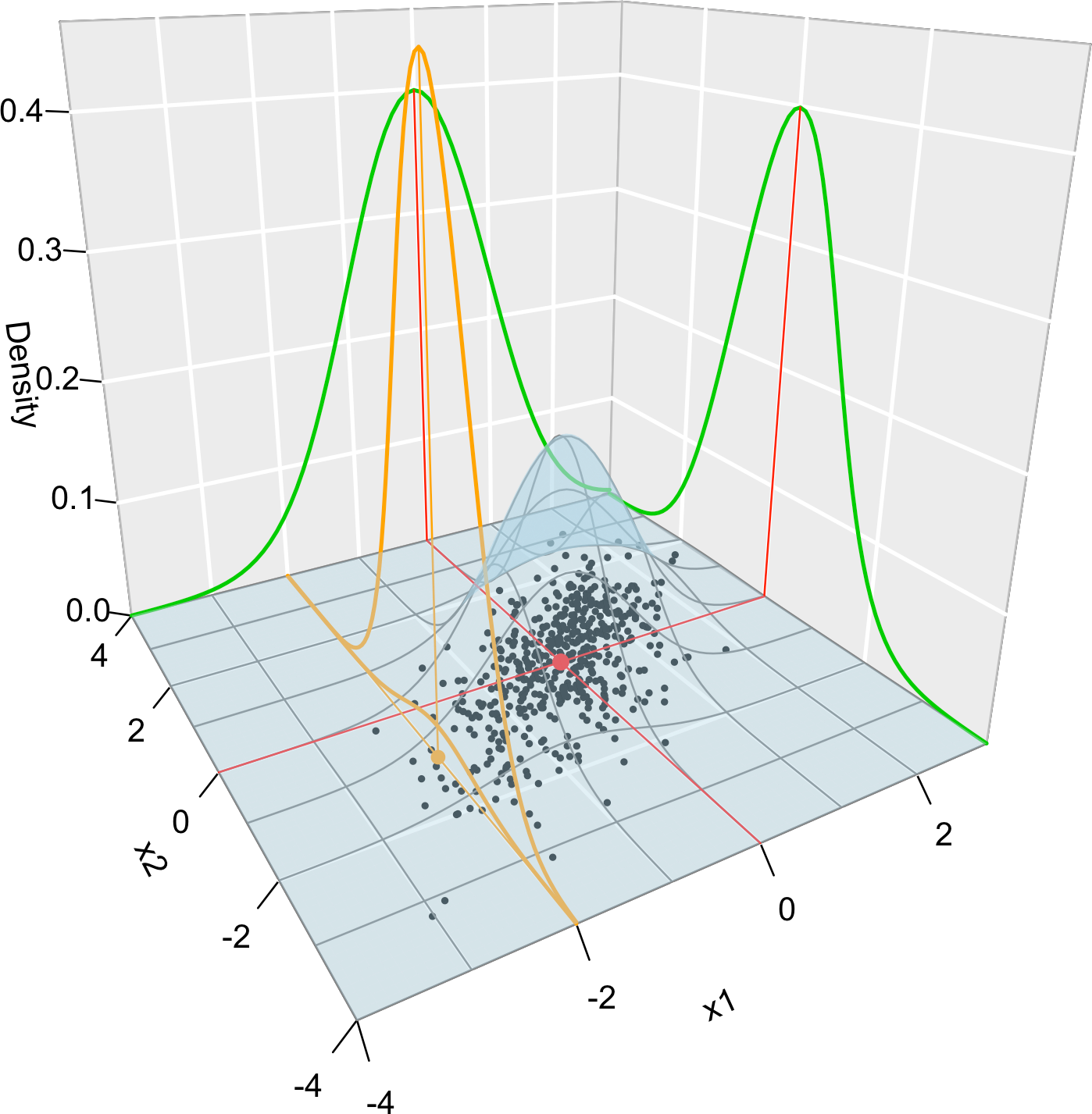
Figure 1.1: Visualization of the joint pdf (in blue), marginal pdfs (green), conditional pdf of \(X_2| X_1=x_1\) (orange), expectation (red point), and conditional expectation \(\mathbb{E}\lbrack X_2 | X_1=x_1 \rbrack\) (orange point) of a \(2\)-dimensional normal. The conditioning point of \(X_1\) is \(x_1=-2.\) Note the different scales of the densities, as they have to integrate to one over different supports. Note how the conditional density (upper orange curve) is not the joint pdf \(f(x_1,x_2)\) (lower orange curve) with \(x_1=-2\) but its rescaling by \(\frac{1}{f_{X_1}(x_1)}.\) The parameters of the \(2\)-dimensional normal are \(\mu_1=\mu_2=0,\) \(\sigma_1=\sigma_2=1\) and \(\rho=0.75\) (see Exercise 1.9). \(500\) observations sampled from the distribution are shown in black.
Exercise 1.2 Consider the random vector \((X,Y)\) with joint pdf \[\begin{align*} f(x,y)=\begin{cases} y e^{-a x y},&x>0,\,y\in(0, b),\\ 0,&\text{else.} \end{cases} \end{align*}\]
- Determine the value of \(b>0\) that makes \(f\) a valid pdf.
- Compute \(\mathbb{E}[X]\) and \(\mathbb{E}[Y].\)
- Verify the law of the total expectation.
- Verify the law of the total variance.
Exercise 1.3 Consider the continuous random vector \((X_1,X_2)\) with joint pdf given by
\[\begin{align*} f(x_1,x_2)=\begin{cases} 2,&0<x_1<x_2<1,\\ 0,&\mathrm{else.} \end{cases} \end{align*}\]
- Check that \(f\) is a proper pdf.
- Obtain the joint cdf of \((X_1,X_2).\)
- Obtain the marginal pdfs of \(X_1\) and \(X_2.\)
- Obtain the marginal cdfs of \(X_1\) and \(X_2.\)
- Obtain the conditional pdfs of \(X_1|X_2=x_2\) and \(X_2|X_1=x_1.\)
1.1.5 Variance-covariance matrix
For two random variables \(X_1\) and \(X_2,\) the covariance between them is defined as
\[\begin{align*} \mathrm{Cov}[X_1,X_2]:=\mathbb{E}[(X_1-\mathbb{E}[X_1])(X_2-\mathbb{E}[X_2])]=\mathbb{E}[X_1X_2]-\mathbb{E}[X_1]\mathbb{E}[X_2], \end{align*}\]
and the correlation between them, as
\[\begin{align*} \mathrm{Cor}[X_1,X_2]:=\frac{\mathrm{Cov}[X_1,X_2]}{\sqrt{\mathbb{V}\mathrm{ar}[X_1]\mathbb{V}\mathrm{ar}[X_2]}}. \end{align*}\]
The variance and the covariance are extended to a random vector \(\mathbf{X}=(X_1,\ldots,X_p)'\) by means of the so-called variance-covariance matrix:
\[\begin{align*} \mathbb{V}\mathrm{ar}[\mathbf{X}]:=&\,\mathbb{E}[(\mathbf{X}-\mathbb{E}[\mathbf{X}])(\mathbf{X}-\mathbb{E}[\mathbf{X}])']\\ =&\,\mathbb{E}[\mathbf{X}\mathbf{X}']-\mathbb{E}[\mathbf{X}]\mathbb{E}[\mathbf{X}]'\\ =&\,\begin{pmatrix} \mathbb{V}\mathrm{ar}[X_1] & \mathrm{Cov}[X_1,X_2] & \cdots & \mathrm{Cov}[X_1,X_p]\\ \mathrm{Cov}[X_2,X_1] & \mathbb{V}\mathrm{ar}[X_2] & \cdots & \mathrm{Cov}[X_2,X_p]\\ \vdots & \vdots & \ddots & \vdots \\ \mathrm{Cov}[X_p,X_1] & \mathrm{Cov}[X_p,X_2] & \cdots & \mathbb{V}\mathrm{ar}[X_p]\\ \end{pmatrix}, \end{align*}\]
where \(\mathbb{E}[\mathbf{X}]:=(\mathbb{E}[X_1],\ldots,\mathbb{E}[X_p])'\) is just the componentwise expectation. As in the univariate case, the expectation is a linear operator, which now means that
\[\begin{align} \mathbb{E}[\mathbf{A}\mathbf{X}+\mathbf{b}]=\mathbf{A}\mathbb{E}[\mathbf{X}]+\mathbf{b},\quad\text{for a $q\times p$ matrix } \mathbf{A}\text{ and }\mathbf{b}\in\mathbb{R}^q.\tag{1.2} \end{align}\]
It follows from (1.2) that
\[\begin{align} \mathbb{V}\mathrm{ar}[\mathbf{A}\mathbf{X}+\mathbf{b}]=\mathbf{A}\mathbb{V}\mathrm{ar}[\mathbf{X}]\mathbf{A}',\quad\text{for a $q\times p$ matrix } \mathbf{A}\text{ and }\mathbf{b}\in\mathbb{R}^q.\tag{1.3} \end{align}\]
1.1.6 Inequalities
We conclude this section by reviewing some useful probabilistic inequalities.
Proposition 1.2 (Markov's inequality) Let \(X\) be a nonnegative random variable with \(\mathbb{E}[X]<\infty.\) Then
\[\begin{align*} \mathbb{P}[X\geq t]\leq\frac{\mathbb{E}[X]}{t}, \quad\forall t>0. \end{align*}\]
Proposition 1.3 (Chebyshev's inequality) Let \(X\) be a random variable with \(\mu=\mathbb{E}[X]\) and \(\sigma^2=\mathbb{V}\mathrm{ar}[X]<\infty.\) Then
\[\begin{align*} \mathbb{P}[|X-\mu|\geq t]\leq\frac{\sigma^2}{t^2},\quad \forall t>0. \end{align*}\]
Exercise 1.4 Prove Markov’s inequality using \(X=X1_{\{X\geq t\}}+X1_{\{X< t\}}.\)
Exercise 1.5 Prove Chebyshev’s inequality using Markov’s.
Remark. Chebyshev’s inequality gives a quick and handy way of computing confidence intervals for the values of any random variable \(X\) with finite variance:
\[\begin{align} \mathbb{P}[X\in(\mu-t\sigma, \mu+t\sigma)]\geq 1-\frac{1}{t^2},\quad \forall t>0.\tag{1.4} \end{align}\]
That is, for any \(t>0,\) the interval \((\mu-t\sigma, \mu+t\sigma)\) has, at least, a probability \(1-1/t^2\) of containing a random realization of \(X.\) The intervals are conservative, but extremely general. The table below gives the guaranteed coverage probability \(1-1/t^2\) for common values of \(t.\)
| \(t\) | \(2\) | \(3\) | \(4\) | \(5\) | \(6\) |
|---|---|---|---|---|---|
| Guaranteed coverage | \(0.75\) | \(0.8889\) | \(0.9375\) | \(0.96\) | \(0.9722\) |
Exercise 1.6 Prove (1.4) from Chebyshev’s inequality.
Proposition 1.4 (Cauchy–Schwartz inequality) Let \(X\) and \(Y\) such that \(\mathbb{E}[X^2]<\infty\) and \(\mathbb{E}[Y^2]<\infty.\) Then
\[\begin{align*} |\mathbb{E}[XY]|\leq\sqrt{\mathbb{E}[X^2]\mathbb{E}[Y^2]}. \end{align*}\]
Exercise 1.7 Prove Cauchy–Schwartz inequality “pulling a rabbit out of a hat”: consider the polynomial \(p(t)=\mathbb{E}[(tX+Y)^2]=At^2+2Bt+C\geq0,\) \(\forall t\in\mathbb{R}.\)
Exercise 1.8 Does \(\mathbb{E}[|XY|]\leq\sqrt{\mathbb{E}[X^2]\mathbb{E}[Y^2]}\) hold? Observe that, due to the next proposition, \(|\mathbb{E}[XY]|\leq \mathbb{E}[|XY|].\)
Proposition 1.5 (Jensen's inequality) If \(g\) is a convex function, then
\[\begin{align*} g(\mathbb{E}[X])\leq\mathbb{E}[g(X)]. \end{align*}\]
Example 1.1 Jensen’s inequality has interesting derivations. For example:
- Take \(h=-g.\) Then \(h\) is a concave function and \(h(\mathbb{E}[X])\geq\mathbb{E}[h(X)].\)
- Take \(g(x)=|x|^r\) for \(r\geq 1,\) which is a convex function. Then \(|\mathbb{E}[X]|^r\leq \mathbb{E}[|X|^r].\) If \(0<r<1,\) then \(g(x)=|x|^r\) is concave and \(|\mathbb{E}[X]|^r\geq \mathbb{E}[|X|^r].\)
- Consider \(0<r\leq s.\) Then \(g(x)=|x|^{s/r}\) is convex (since \(s/r\geq 1\)) and \(g(\mathbb{E}[|X|^r])\leq \mathbb{E}[g(|X|^r)]=\mathbb{E}[|X|^s].\) As a consequence, \(\mathbb{E}[|X|^s]<\infty\implies\mathbb{E}[|X|^r]<\infty\) for \(0\leq r\leq s.\)5
- The exponential (logarithm) function is convex (concave). Consequently, \(\exp(\mathbb{E}[X])\leq\mathbb{E}[\exp(X)]\) and \(\log(\mathbb{E}[|X|])\geq\mathbb{E}[\log(|X|)].\)