4.4 Regressogram

The regressogram is the adaptation of the histogram to the regression setting. Historically, it has received attention in several applied areas.¹⁵⁸ This and its connection with the histogram are the reasons for its inclusion in the notes, since its performance to estimate $m$ is definitely inferior to that of $\hat{m}(\cdot;p,h)$ (see Figure 4.4). The construction described below can be regarded as the opposite path to the one followed in Sections 2.1–2.2 for constructing the kde from the histogram: now we deconstruct the Nadaraya–Watson estimator to obtain the regressogram.

Based on (4.2), the Nadaraya–Watson estimator was constructed by plugging kdes for the joint density of $(X,Y)$ and the marginal density of $X.$ This resulted in

\[\begin{align} \hat{m}(x;0,h)=\frac{\sum_{i=1}^nK_h(x-X_i)Y_i}{\sum_{i=1}^nK_h(x-X_i)}=\frac{\frac{1}{n}\sum_{i=1}^nK_h(x-X_i)Y_i}{\hat{f}(x;h)},\tag{4.26} \end{align}\]

which clearly emphasizes the connection between the kde $\hat{f}(x;h)=\frac{1}{n}\sum_{i=1}^nK_h(x-X_i)$ and $\hat{m}(x;0,h).$ Evidently, this approach gives a smooth estimator for the regression function if the kernels employed in the kde are smooth.

Within (4.26), a possibility is to consider the uniform kernel $K(z)=\frac{1}{2}1_{\{-1<x<1\}}$ in the kde¹⁵⁹, which results in

\[\begin{align} \hat{m}_\mathrm{N}(x;h):=\frac{\sum_{i=1}^n1_{\{X_i-h<x<X_i+h\}}Y_i}{\sum_{i=1}^n1_{\{X_i-h<x<X_i+h\}}}=\frac{1}{|N(x;h)|}\sum_{i\in N(x;h)}Y_i,\tag{4.27} \end{align}\]

where $N(x;h):=\{i=1,\ldots,n:|X_i-x|<h\}$ is the set of the indexes of the sample within the neighborhood of $x$ and $|N(x;h)|$ denotes its size.¹⁶⁰ Estimator (4.27), a naive regression estimator, is precisely the regression analogue of the moving histogram or naive density estimator. Its second expression in (4.27) reveals that it is just a sample mean in different blocks (or neighborhoods) of the data. As a consequence, it is discontinuous.

Another alternative to the kde in (4.26) is to employ the histogram $\hat{f}_\mathrm{H}(x;t_0,h)=\frac{1}{nh}\sum_{i=1}^n1_{\{X_i\in B_k:x\in B_k\}},$ where $\{B_k=[t_{k},t_{k+1}):t_k=t_0+hk,k\in\mathbb{Z}\}$ (recall Section 2.1.1). This yields the regressogram of $m$:

\[\begin{align} \hat{m}_\mathrm{R}(x;h):=\frac{\sum_{i=1}^n1_{\{X_i\in B_k\}}Y_i}{\sum_{i=1}^n1_{\{X_i\in B_k\}}}=\frac{1}{|B(k;h)|}\sum_{i\in B(k;h)}Y_i,\quad\text{if }x\in B_k,\tag{4.28} \end{align}\]

where $B(k;h):=\{i=1,\ldots,n:X_i\in B_k\}$ and $|B(k;h)|$ stands for its size (denoted by $v_k$ in Section 2.1.1). The difference of the regressogram with respect to the naive regression estimator is that the former pre-defines fixed bins in which to compute the bin means, producing a final estimator that, for the same bandwidth $h,$ is notably more rigid (it is constant on each bin $B_k;$ see Figure 4.4).

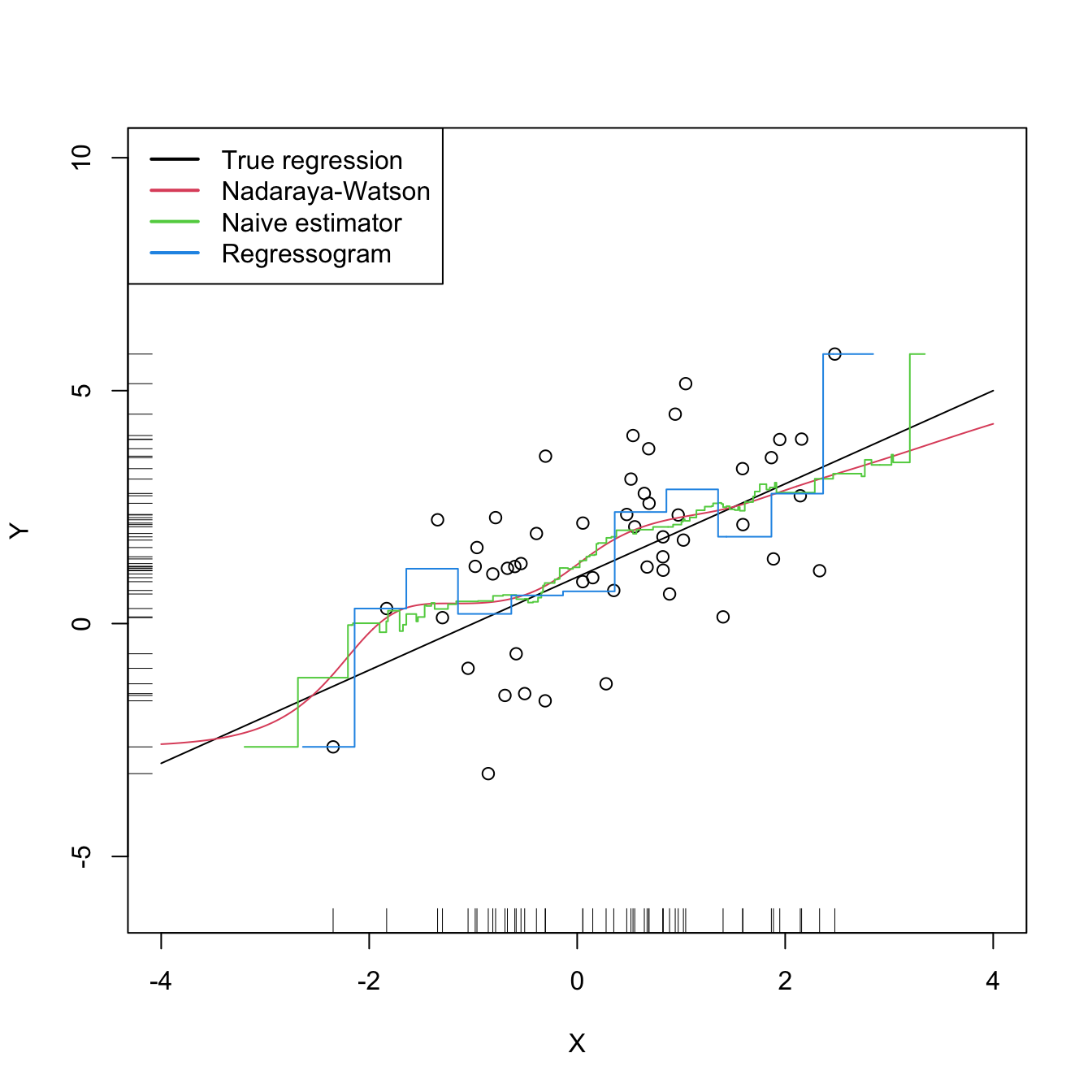
$The Nadaraya–Watson estimator, the naive regression estimator, and the regressogram. Notice that the naive regression estimator and the regressogram are not defined everywhere – only for those regions in which there are nearby observations of $X.$ All the estimators share the bandwidth $h=0.5,$ a fair comparison since the scaled uniform kernel, $\tilde K(z)=\frac{1}{2\sqrt{3}}1_{\{-\sqrt{3}<z<\sqrt{3}\}},$ is employed for the naive estimator. The regressogram employs $t_0=0.$ The regression setting is explained in Exercise 4.16.$

Figure 4.4: The Nadaraya–Watson estimator, the naive regression estimator, and the regressogram. Notice that the naive regression estimator and the regressogram are not defined everywhere – only for those regions in which there are nearby observations of $X.$ All the estimators share the bandwidth $h=0.5,$ a fair comparison since the scaled uniform kernel, $\tilde K(z)=\frac{1}{2\sqrt{3}}1_{\{-\sqrt{3}<z<\sqrt{3}\}},$ is employed for the naive estimator. The regressogram employs $t_0=0.$ The regression setting is explained in Exercise 4.16.

Exercise 4.16 Implement in R your own version of the naive regression estimator (4.27). It must be a function that takes as inputs:

a vector with the evaluation points $x,$
a sample $(X_1,Y_1),\ldots,(X_n,Y_n),$
a bandwidth $h,$

and that returns (4.27) evaluated for each $x.$ Test the implementation by estimating the regression function $m(x)=1+x$ for the regression model $Y=m(X)+\varepsilon,$ where $X\sim\mathcal{N}(0, 1)$ and $\varepsilon\sim\mathcal{N}(0,2)$ using $n=50$ observations. This is the setting used in Figure 4.4.

Exercise 4.17 Perform Exercise 4.16 by implementing in R the regressogram (4.28) instead of the naive regression estimator. The R function must now have an additional argument $t_0.$

References

ESA. 1997. The Hipparcos and Tycho Catalogues. Vol. 1200. ESA SP. Noordwijk: ESA Publication Division. https://doi.org/https://www.cosmos.esa.int/web/hipparcos/catalogues.

For example, in astronomy, check Figure 3.2.17 in Vol. 1 in ESA (1997).↩︎
Equivalently, the naive density estimator $\hat{f}_\mathrm{N}(x;h)=\frac{1}{2nh}\sum_{i=1}^n1_{\{x-h<X_i<x+h\}}$ instead of the kde.↩︎
Observe that (4.27) is defined only for $x$ such that $|N(x;h)|>0.$ It is perfectly possible to have $|N(x;h)|=0$ in practice. This does not happen for non-compactly supported kernels, for which $N(x;h)=\mathbb{R}$ for any $x,$ $h,$ and sample arrangement.↩︎