1.4 \(O_\mathbb{P}\) and \(o_\mathbb{P}\) notation
1.4.1 Deterministic versions
In computer science the \(O\) notation is used to measure the complexity of algorithms. For example, when an algorithm is \(O(n^2),\) it is said that it is quadratic in time and we know that is going to take on the order of \(n^2\) operations to process an input of size \(n.\) We do not care about the specific amount of computations; rather, we focus on the big picture by looking for an upper bound for the sequence of computation times in terms of \(n.\) This upper bound disregards constants. For example, the dot product between two vectors of size \(n\) is an \(O(n)\) operation, although it takes \(n\) multiplications and \(n-1\) sums, hence \(2n-1\) operations. In essence, the \(O\) notation allows us to trade precision for simplicity.
In mathematical analysis, \(O\)-related notation is mostly used to bound sequences that shrink to zero. This is the use we will be concerned about. The technicalities are the same, but the use of the notation is slightly different.
Definition 1.5 (Big-\(O\)) Given two strictly positive sequences \(a_n\) and \(b_n,\)
\[\begin{align*} a_n=O(b_n)\,:\!\iff \limsup_{n\to\infty}\frac{a_n}{b_n}\leq C,\text{ for a }C>0. \end{align*}\]
If \(a_n=O(b_n),\) then we say that \(a_n\) is big-\(O\) of \(b_n.\) To indicate that \(a_n\) is bounded, we write \(a_n=O(1).\)11
Definition 1.6 (Little-\(o\)) Given two strictly positive sequences \(a_n\) and \(b_n,\)
\[\begin{align*} a_n=o(b_n)\,:\!\iff \lim_{n\to\infty}\frac{a_n}{b_n}=0. \end{align*}\]
If \(a_n=o(b_n),\) then we say that \(a_n\) is little-\(o\) of \(b_n.\) To indicate that \(a_n\to0,\) we write \(a_n=o(1).\)
Remark. An immediate but important consequence of the big-\(O\) and little-\(o\) definitions is that
\[\begin{align} a_n=O(b_n)\!\iff \frac{a_n}{b_n}=O(1) \text{ and } a_n=o(b_n)\!\iff \frac{a_n}{b_n}=o(1). \tag{1.7} \end{align}\]
Exercise 1.11 Show the following statements by directly applying the previous definitions.
- \(n^{-2}=o(n^{-1}).\)
- \(\log n=O(n).\)
- \(n^{-1}=o((\log n)^{-1}).\)
- \(n^{-4/5}=o(n^{-2/3}).\)
- \(3\sin(n)=O(1).\)
- \(n^{-2}-n^{-3}+n^{-1}=O(n^{-1}).\)
- \(n^{-2}-n^{-3}=o(n^{-1/2}).\)
The interpretation of these two definitions is simple:12
- \(a_n=O(b_n)\) means that \(a_n\) is “not larger than” \(b_n\) asymptotically. If \(a_n,b_n\to0,\) then it means that \(a_n\) “decreases as fast or faster” than \(b_n.\)
- \(a_n=o(b_n)\) means that \(a_n\) is “smaller than” \(b_n\) asymptotically. If \(a_n,b_n\to0,\) then it means that \(a_n\) “decreases faster” than \(b_n.\)
Obviously, little-\(o\) implies big-\(O\) (take any \(C>0\) in Definition 1.5). Playing with limits we can get a list of useful facts.
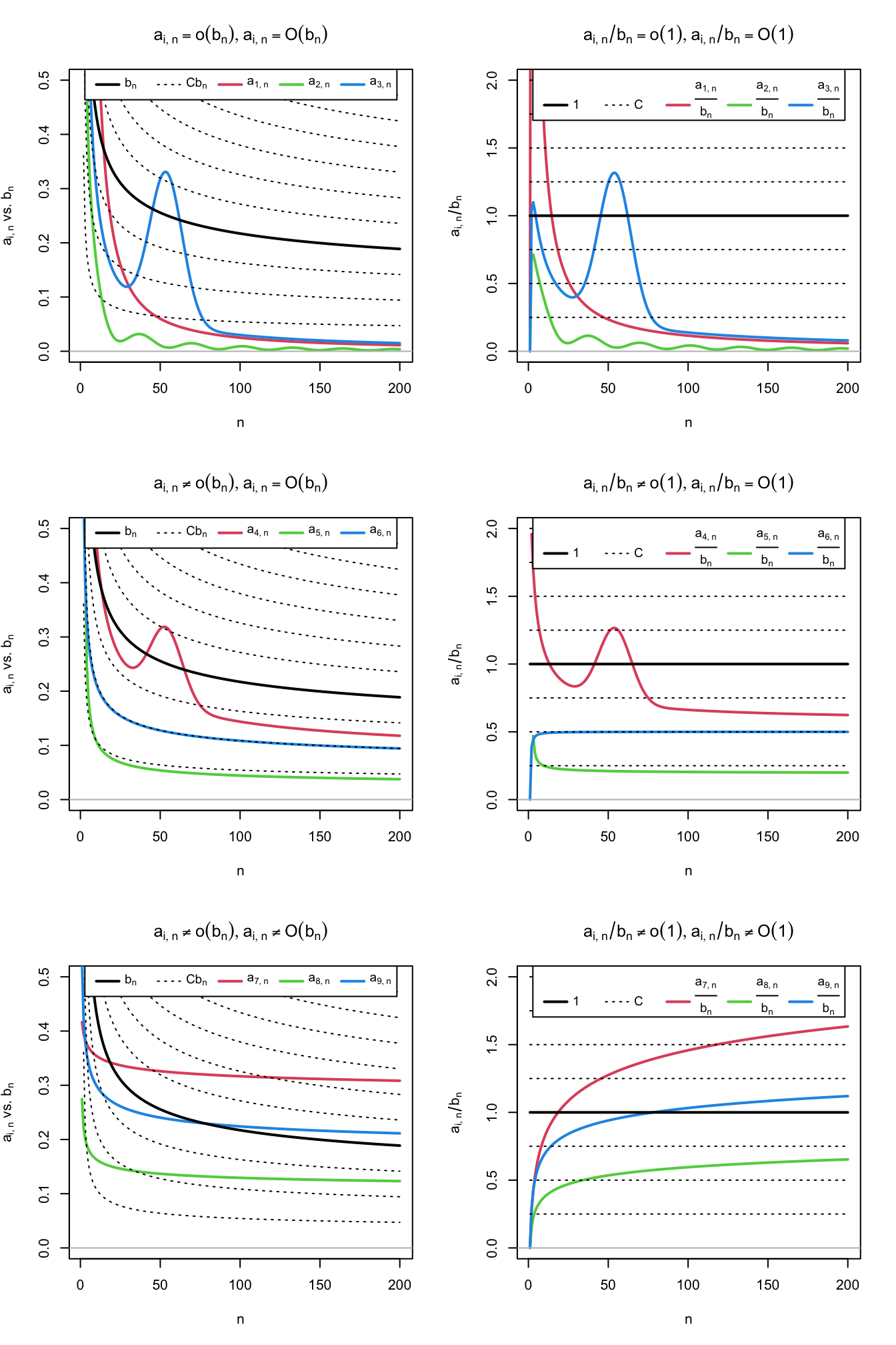
Figure 1.2: Differences and similarities between little-\(o\) and big-\(O,\) illustrated for the dominating sequence \(b_n=1/\log(n)\) (black solid curve) and sequences \(a_{i,n},\) \(j=1,\ldots,9\) (colored curves). The dashed lines represent the sequences \(Cb_n,\) for a grid of constants \(C.\) The plots on the left column compare \(a_{i,n}\) against \(b_n,\) whereas the right column plots show the equivalent view in terms of the ratios \(a_{i,n}/b_n\) (recall (1.7)). Sequences \(a_{1,n}=2 / n + 50 / n^2,\) \(a_{2,n}=(\sin(n/5) + 2) / n^{5/4},\) and \(a_{3,n}=3(1 + 5 \exp(-(n - 55.5)^2 / 200)) / n\) are \(o(b_n)\) (hence also \(O(b_n)\)). Sequences \(a_{4,n}=(2\log_{10}(n)((n + 3) / (2n)))^{-1} + a_{3,n}/2,\) \(a_{5,n}=(4\log_2(n/2))^{-1},\) and \(a_{6,n}=(\log(n^2 + n))^{-1}\) are \(O(b_n),\) but not \(o(b_n).\) Finally, sequences \(a_{7,n}=\log(5n + 3)^{-1/4}/2,\) \(a_{8,n}=(4\log(\log(10n + 2)))^{-1},\) and \(a_{9,n}=(2\log(\log(n^2 + 10n + 2)))^{-1}\) are not \(O(b_n)\) (hence neither \(o(b_n)\)).
Proposition 1.7 Consider two strictly positive sequences \(a_n,b_n\to0.\) The following properties hold:
- \(kO(a_n)=O(a_n),\) \(ko(a_n)=o(a_n),\) \(k\in\mathbb{R}.\)
- \(o(a_n)+o(b_n)=o(a_n+b_n),\) \(O(a_n)+O(b_n)=O(a_n+b_n).\)
- \(o(a_n)o(b_n)=o(a_nb_n),\) \(O(a_n)O(b_n)=O(a_nb_n).\)
- \(o(a_n)+O(b_n)=O(a_n+b_n),\) \(o(a_n)O(b_n)=o(a_nb_n).\)
- \(o(1)O(a_n)=o(a_n).\)
- \(a_n^r=o(a_n^s),\) for \(r>s\geq 0.\)
- \(a_nb_n=o(a_n+b_n).\)
- \((a_n+b_n)^k=O(a_n^k+b_n^k).\)
The last result is a consequence of a useful inequality.
Lemma 1.1 (\(C_p\) inequality) Given \(a,b\in\mathbb{R}\) and \(p>0,\)
\[\begin{align*} |a+b|^p\leq C_p(|a|^p+|b|^p), \quad C_p=\begin{cases} 1,&p\leq1,\\ 2^{p-1},&p>1. \end{cases} \end{align*}\]
Exercise 1.12 Illustrate the properties of Proposition 1.7 considering \(a_n=n^{-1}\) and \(b_n=n^{-1/2}.\)
1.4.2 Stochastic versions
The previous notation is purely deterministic. Let’s add some stochastic flavor by establishing the stochastic analogous of little-\(o.\)
Definition 1.7 (Little-\(o_\mathbb{P}\)) Given a strictly positive sequence \(a_n\) and a sequence of random variables \(X_n,\)
\[\begin{align*} X_n=o_\mathbb{P}(a_n)\,:\!\iff& \frac{|X_n|}{a_n}\stackrel{\mathbb{P}}{\longrightarrow}0 \\ \iff& \lim_{n\to\infty}\mathbb{P}\left[\frac{|X_n|}{a_n}>\varepsilon\right]=0,\;\forall\varepsilon>0. \end{align*}\]
If \(X_n=o_\mathbb{P}(a_n),\) then we say that \(X_n\) is little-\(o_\mathbb{P}\) of \(a_n.\) To indicate that \(X_n\stackrel{\mathbb{P}}{\longrightarrow}0,\) we write \(X_n=o_\mathbb{P}(1).\)
Therefore, little-\(o_\mathbb{P}\) allows us to easily quantify the speed at which a sequence of random variables converges to zero in probability.
Example 1.3 Let \(Y_n=o_\mathbb{P}\big(n^{-1/2}\big)\) and \(Z_n=o_\mathbb{P}(n^{-1}).\) Then \(Z_n\) converges faster to zero in probability than \(Y_n.\) To visualize this, recall that \(X_n=o_\mathbb{P}(a_n)\) and that limit definitions entail that
\[\begin{align*} \forall\varepsilon,\delta>0,\,\exists \,n_0=n_0(\varepsilon,\delta)\in\mathbb{N}:\forall n\geq n_0(\varepsilon,\delta),\, \mathbb{P}\left[|X_n|>a_n\varepsilon\right]<\delta. \end{align*}\]
Therefore, for fixed \(\varepsilon,\delta>0\) and a fixed \(n\geq\max(n_{0,Y},n_{0,Z}),\) then \(\mathbb{P}\left[Y_n\in\big(-n^{-1/2}\varepsilon,n^{-1/2}\varepsilon\big)\right]>1-\delta\) and \(\mathbb{P}\left[Z_n\in(-n^{-1}\varepsilon,n^{-1}\varepsilon)\right]>1-\delta,\) but the latter interval is much shorter, hence \(Z_n\) is forced to be more tightly concentrated about \(0.\)
Big-\(O_\mathbb{P}\) allows us to bound a sequence of random variables in probability, in the sense that we can state that the probability of being above an arbitrarily large threshold \(C\) converges to zero. As with its deterministic versions \(o\) and \(O,\) a little-\(o_\mathbb{P}\) is more restrictive than a big-\(O_\mathbb{P}\), and the former implies the latter.
Definition 1.8 (Big-\(O_\mathbb{P}\)) Given a strictly positive sequence \(a_n\) and a sequence of random variables \(X_n,\)
\[\begin{align*} X_n=O_\mathbb{P}(a_n)\,:\!\iff&\forall\varepsilon>0,\,\exists\,C_\varepsilon>0,\,n_0(\varepsilon)\in\mathbb{N}:\\ &\forall n\geq n_0(\varepsilon),\, \mathbb{P}\left[\frac{|X_n|}{a_n}>C_\varepsilon\right]<\varepsilon\\ \iff& \lim_{C\to\infty}\limsup_{n\to\infty}\mathbb{P}\left[\frac{|X_n|}{a_n}>C\right]=0. \end{align*}\]
If \(X_n=O_\mathbb{P}(a_n),\) then we say that \(X_n\) is big-\(O_\mathbb{P}\) of \(a_n.\)
Remark. An immediate but important consequence of the big-\(O_\mathbb{P}\) and little-\(o_\mathbb{P}\) definitions is that
\[\begin{align} X_n=O_\mathbb{P}(a_n)\!\iff \frac{X_n}{a_n}=O_\mathbb{P}(1) \text{ and } X_n=o_\mathbb{P}(a_n)\!\iff \frac{X_n}{a_n}=o_\mathbb{P}(1). \tag{1.8} \end{align}\]
Example 1.4 Any sequence of random variables such that \(X_n=X\) for all \(n\geq 1,\) with \(X\) any random variable, is trivially \(X_n=O_\mathbb{P}(1).\) Indeed, it is satisfied that \(\lim_{C\to\infty}\limsup_{n\to\infty}\mathbb{P}\left[\frac{|X_n|}{1}>C\right]=\lim_{C\to\infty}\mathbb{P}[|X_n|>C]=0.\)
Example 1.5 Chebyshev inequality entails that \(\mathbb{P}[|X_n-\mathbb{E}[X_n]|\geq t]\leq \mathbb{V}\mathrm{ar}[X_n]/t^2,\) \(\forall t>0.\) Setting \(\varepsilon:=\mathbb{V}\mathrm{ar}[X_n]/t^2\) and \(C_\varepsilon:=1/\sqrt{\varepsilon},\) then \(\mathbb{P}\left[|X_n-\mathbb{E}[X_n]|\geq \sqrt{\mathbb{V}\mathrm{ar}[X_n]}C_\varepsilon\right]\leq \varepsilon.\) Therefore,
\[\begin{align} X_n-\mathbb{E}[X_n]=O_\mathbb{P}\left(\sqrt{\mathbb{V}\mathrm{ar}[X_n]}\right).\tag{1.9} \end{align}\]
This is a very useful result, as it gives an efficient way of deriving the big-\(O_\mathbb{P}\) form of a sequence of random variables \(X_n\) with finite variances.
An application of Example 1.5 shows that \(X_n=O_\mathbb{P}(n^{-1/2})\) for \(X_n\stackrel{d}{=}\mathcal{N}(0,1/n).\) The nature of this statement and its relation with little-\(o_\mathbb{P}\) is visualized with Figure 1.3, which shows a particular realization \(X_n(\omega)\) of the sequence of random variables.
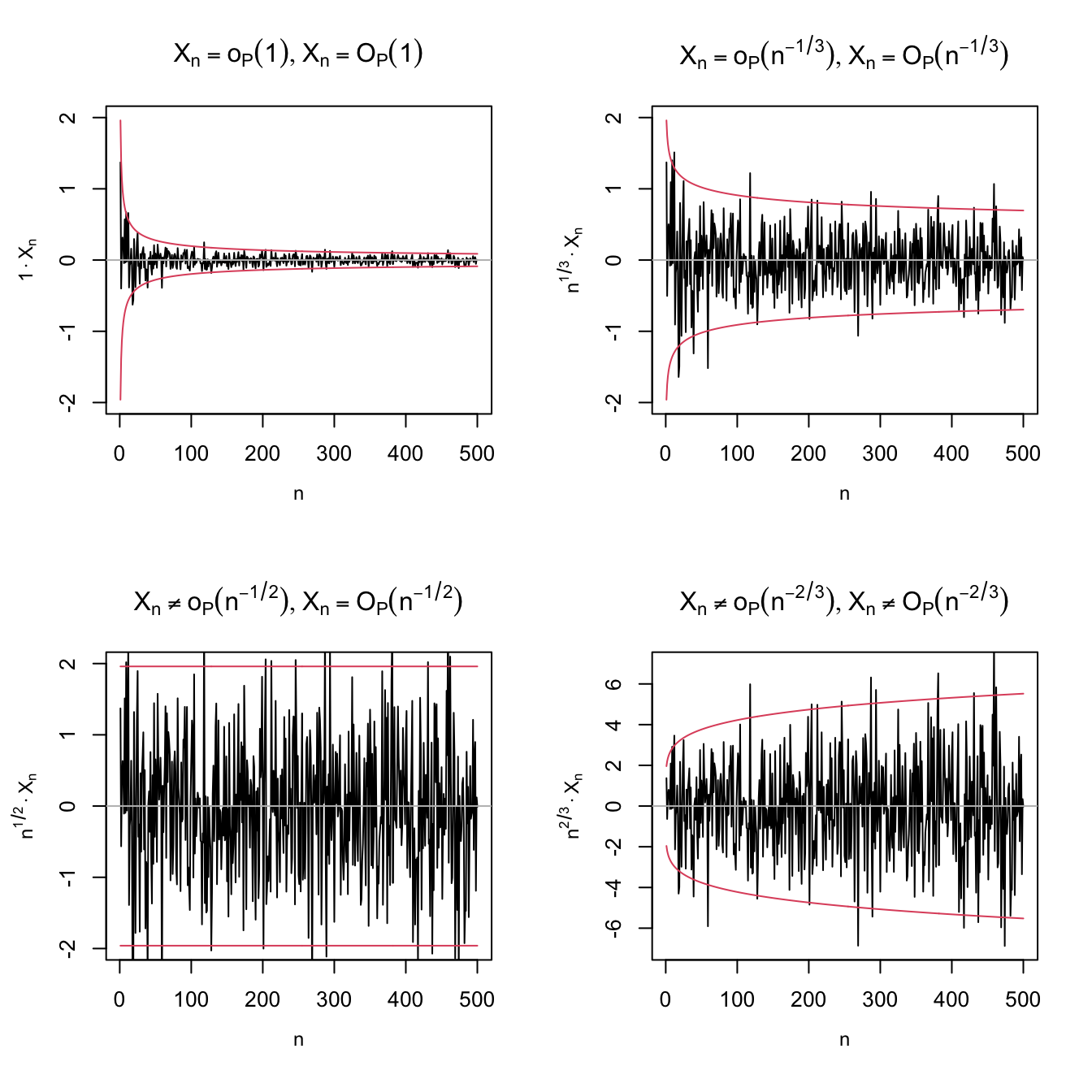
Figure 1.3: Differences and similarities between little-\(o_\mathbb{P}\) and big-\(O_\mathbb{P},\) illustrated for the sequence of random variables \(X_n\stackrel{d}{=}\mathcal{N}(0,1/n).\) Since \(X_n\stackrel{\mathbb{P}}{\longrightarrow}0,\) \(X_n=o_\mathbb{P}(1),\) as evidenced in the upper left plot. The next plots check if \(X_n=o_\mathbb{P}(a_n)\) by evaluating if \(X_n/a_n\stackrel{\mathbb{P}}{\longrightarrow}0\) (recall (1.8)), for \(a_n=n^{-1/3},n^{-1/2},n^{-2/3}.\) Clearly, \(X_n=o_\mathbb{P}(n^{-1/3})\) (\(n^{1/3}X_n\stackrel{\mathbb{P}}{\longrightarrow}0\)) but \(X_n\neq o_\mathbb{P}(n^{-1/2})\) (\(n^{1/2}X_n\stackrel{\mathbb{P}}{\longrightarrow}\mathcal{N}(0,1)\)) and \(X_n\neq o_\mathbb{P}(n^{-2/3})\) (\(n^{2/3}X_n\) diverges). In the first three cases, \(X_n=O_\mathbb{P}(a_n);\) the fourth is \(X_n\neq O_\mathbb{P}(n^{-2/3}),\) \(n^{2/3}X_n\) is not bounded in probability. The red lines represent the \(95\%\) confidence intervals \(\left(-z_{0.025}/(a_n\sqrt{n}),z_{0.025}/(a_n\sqrt{n})\right)\) of the random variable \(X_n/a_n,\) and help evaluating graphically the convergence in probability towards zero.
Exercise 1.13 As illustrated in Figure 1.3, prove that it is actually true that:
- \(X_n\stackrel{\mathbb{P}}{\longrightarrow}0.\)
- \(n^{1/3}X_n\stackrel{\mathbb{P}}{\longrightarrow}0.\)
- \(n^{1/2}X_n\stackrel{\mathbb{P}}{\longrightarrow}\mathcal{N}(0,1).\)
Exercise 1.14 Prove that if \(X_n\stackrel{d}{\longrightarrow}X,\) then \(X_n=O_\mathbb{P}(1).\) Hint: use the double-limit definition and note that \(X=O_\mathbb{P}(1).\)
Example 1.6 (Example 1.18 in DasGupta (2008)) Suppose that \(a_n(X_n-c_n)\stackrel{d}{\longrightarrow}X\) for deterministic sequences \(a_n\) and \(c_n\) such that \(c_n\to c.\) Then, if \(a_n\to\infty,\) \(X_n-c=o_\mathbb{P}(1).\) The argument is simple:
\[\begin{align*} X_n-c&=X_n-c_n+c_n-c\\ &=\frac{1}{a_n}a_n(X_n-c_n)+o(1)\\ &=\frac{1}{a_n}O_\mathbb{P}(1)+o(1). \end{align*}\]
Exercise 1.15 Using the previous example, derive the weak law of large numbers as a consequence of the CLT, both for id and non-id independent random variables.
Proposition 1.8 Consider two strictly positive sequences \(a_n,b_n\to 0.\) The following properties hold:
- \(o_\mathbb{P}(a_n)=O_\mathbb{P}(a_n)\) (little-\(o_\mathbb{P}\) implies big-\(O_\mathbb{P}\)).
- \(o(1)=o_\mathbb{P}(1),\) \(O(1)=O_\mathbb{P}(1)\) (deterministic implies probabilistic).
- \(kO_\mathbb{P}(a_n)=O_\mathbb{P}(a_n),\) \(ko_\mathbb{P}(a_n)=o_\mathbb{P}(a_n),\) \(k\in\mathbb{R}.\)
- \(o_\mathbb{P}(a_n)+o_\mathbb{P}(b_n)=o_\mathbb{P}(a_n+b_n),\) \(O_\mathbb{P}(a_n)+O_\mathbb{P}(b_n)=O_\mathbb{P}(a_n+b_n).\)
- \(o_\mathbb{P}(a_n)o_\mathbb{P}(b_n)=o_\mathbb{P}(a_nb_n),\) \(O_\mathbb{P}(a_n)O_\mathbb{P}(b_n)=O_\mathbb{P}(a_nb_n).\)
- \(o_\mathbb{P}(a_n)+O_\mathbb{P}(b_n)=O_\mathbb{P}(a_n+b_n),\) \(o_\mathbb{P}(a_n)O_\mathbb{P}(b_n)=o_\mathbb{P}(a_nb_n).\)
- \(o_\mathbb{P}(1)O_\mathbb{P}(a_n)=o_\mathbb{P}(a_n).\)
- \((1+o_\mathbb{P}(1))^{-1}=O_\mathbb{P}(1).\)
Example 1.7 Example 1.5 allows us to obtain the \(O_\mathbb{P}\)-part of a sequence of random variables \(X_n\) with finite variances using (1.9). As a result of ii and iv in Proposition 1.8, we can also further simplify the coarse-grained description of \(X_n\) as
\[\begin{align*} X_n&=O(\mathbb{E}[X_n])+O_\mathbb{P}\left(\sqrt{\mathbb{V}\mathrm{ar}[X_n]}\right)\\ &=O_\mathbb{P}\left(\mathbb{E}[X_n]+\sqrt{\mathbb{V}\mathrm{ar}[X_n]}\right). \end{align*}\]
Exercise 1.16 Consider the following sequences of random variables:
- \(X_n\stackrel{d}{=}\Gamma(n+1,2n)-2.\)
- \(X_n\stackrel{d}{=}\mathrm{B}(n,1/n)-1.\)
- \(X_n\stackrel{d}{=}\mathcal{LN}(0,n^{-1})-\exp((2n)^{-1}).\) Hint: Use that \(e^x=1+x+o(x)\) for \(x\to0.\)
For each \(X_n,\) obtain, if possible, two different positive sequences \(a_n,b_n\to0\) such that:
- \(X_n=o_\mathbb{P}(a_n).\)
- \(X_n\neq o_\mathbb{P}(b_n),\) \(X_n=O_\mathbb{P}(b_n).\)
Use (1.9) and check your results by performing an analogous analysis to that in Figure 1.3.
References
For a deterministic sequence \(a_n,\) \(\limsup_{n\to\infty}a_n:=\lim_{n\to\infty}\left(\sup_{k\geq n}a_k\right)\) is the largest limit of the subsequences of \(a_n.\) It can be defined even if \(\lim_{n\to\infty}a_n\) does not exist (e.g., in trigonometric functions). If \(\lim_{n\to\infty}a_n\) exists, as in most of the common usages of the big-\(O\) notation, then \(\limsup_{n\to\infty}a_n=\lim_{n\to\infty}a_n.\)↩︎
For further intuition, we can regard \(a_n\) and \(b_n\) as two vehicles moving towards “zero”, a far away destination, with \(n\) indexing the time. The faster vehicle is the one that approaches zero faster. If \(a_n=O(b_n),\) then \(a_n\) is as fast or equal to \(b_n.\) If \(a_n=o(b_n),\) then \(a_n\) is strictly faster than \(b_n.\) The comparison is asymptotic, meaning that you focus on what happens on the long run (large \(n\)), disregarding initial differences. In this simplified example, \(\mathrm{plane}_n=O(\mathrm{car}_n)\) and \(\mathrm{car}_n=o(\mathrm{bike}_n)\), despite the fact that initially the car is faster than the plane and the bike can also be faster than the car.↩︎