6.2 Comparison of two distributions

Assume that two iid samples $X_1,\ldots,X_n$ and $Y_1,\ldots,Y_m$ arbitrary distributions $F$ and $G$ are given. We next address the two-sample problem of comparing the unknown distributions $F$ and $G.$

6.2.1 Homogeneity tests

The comparison of $F$ and $G$ can be done by testing their equality, which is known as the testing for homogeneity of the samples $X_1,\ldots,X_n$ and $Y_1,\ldots,Y_m.$ We can therefore address the two-sided hypothesis test

\[\begin{align} H_0:F=G\quad\text{vs.}\quad H_1:F\neq G.\tag{6.13} \end{align}\]

Recall that, differently from the simple and composite hypothesis that appears in goodness-of-fit problems, in the homogeneity problem the null hypothesis $H_0:F=G$ does not specify any form for the distributions $F$ and $G,$ only their equality.

The one-sided hypothesis in which $H_1:F<G$ (or $H_1:F>G$) is also very relevant. Here and henceforth “$F<G$” has a special meaning:

“$F<G$”: there exists at least one $x\in\mathbb{R}$ such that $F(x)<G(x).$²²⁶

Obviously, the alternative $H_1:F<G$ is implied if, for all $x\in\mathbb{R},$

\[\begin{align} F(x)<G(x)&\iff \mathbb{P}[X\leq x]<\mathbb{P}[Y\leq x]\nonumber\\ &\iff \mathbb{P}[X>x]>\mathbb{P}[Y>x].\tag{6.14} \end{align}\]

Consequently, (6.14) means that $X$ produces observations above any fixed threshold $x\in\mathbb{R}$ more likely than $Y$. This concept is known as (strict)²²⁷ stochastic dominance and, precisely, it is said that $X$ is stochastically greater than $Y$ if (6.14) holds.²²⁸

Stochastic dominance is an intuitive concept to interpret $H_1:F<G,$ although it is a stronger statement on the relation of $F$ and $G.$ A more accurate, yet still intuitive, way of regarding $H_1:F<G$ is as a local stochastic dominance: $X$ is stochastically greater than $Y$ only for some specific thresholds $x\in\mathbb{R}.$²²⁹ Figures 6.6 and 6.8 give two examples of presence/absence of stochastic dominance where $H_1:F<G$ holds.

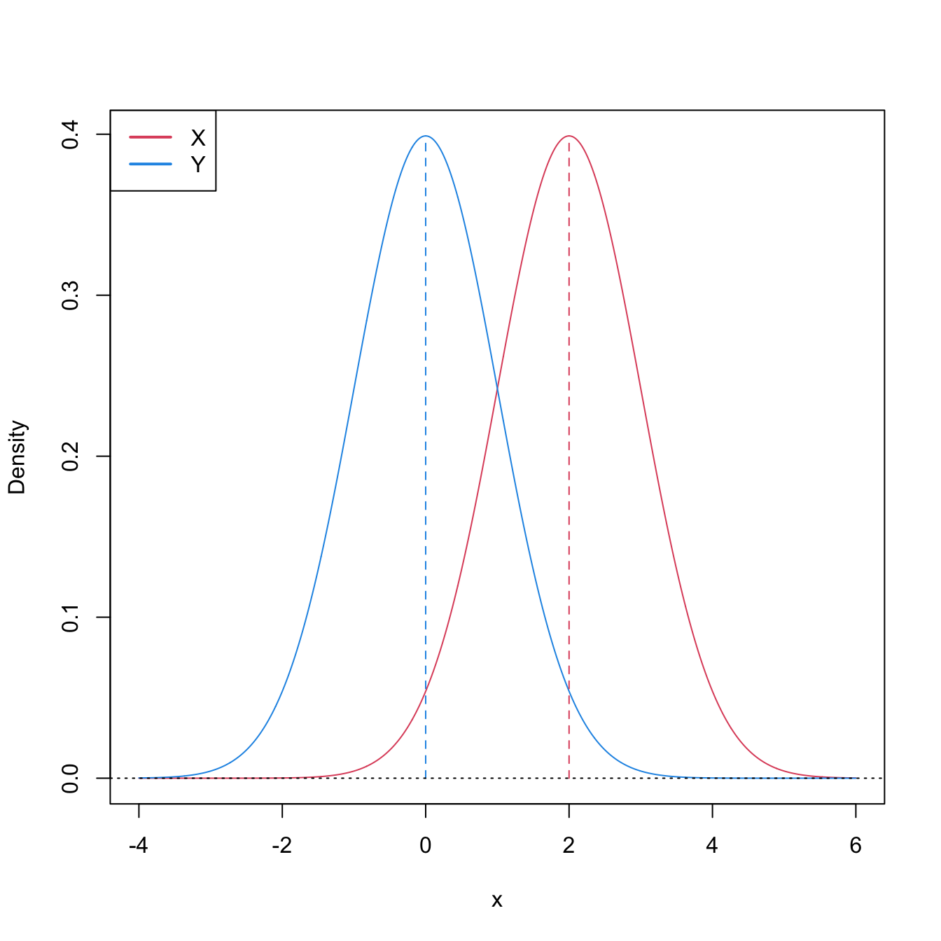
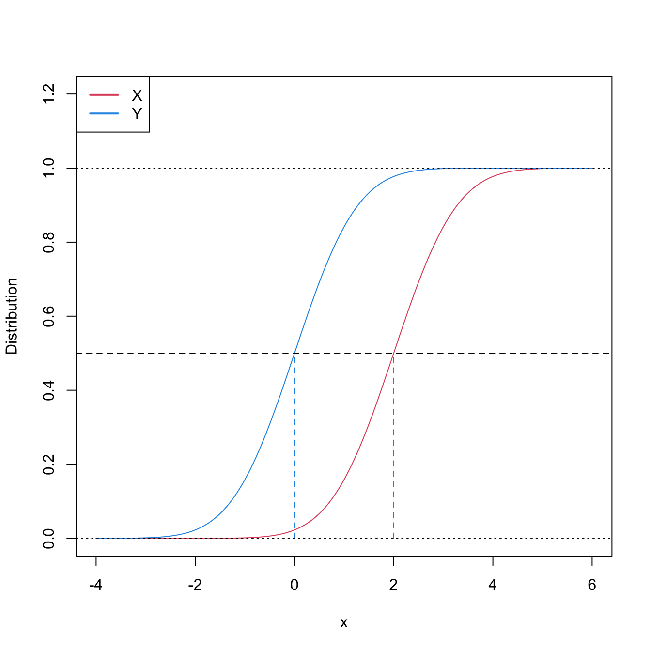
$Pdfs and cdfs of $X\sim\mathcal{N}(2,1)$ and $Y\sim\mathcal{N}(0,1).$ $X$ is stochastically greater than $Y,$ which is visualized in terms of the pdfs (shift in the mean) and cdfs (domination of $Y$’s cdf). The means are shown in solid vertical lines. Note that the variances of $X$ and $Y$ are common; compare this situation with Figure 6.8.$ $Pdfs and cdfs of $X\sim\mathcal{N}(2,1)$ and $Y\sim\mathcal{N}(0,1).$ $X$ is stochastically greater than $Y,$ which is visualized in terms of the pdfs (shift in the mean) and cdfs (domination of $Y$’s cdf). The means are shown in solid vertical lines. Note that the variances of $X$ and $Y$ are common; compare this situation with Figure 6.8.$

Figure 6.6: Pdfs and cdfs of $X\sim\mathcal{N}(2,1)$ and $Y\sim\mathcal{N}(0,1).$ $X$ is stochastically greater than $Y,$ which is visualized in terms of the pdfs (shift in the mean) and cdfs (domination of $Y$’s cdf). The means are shown in solid vertical lines. Note that the variances of $X$ and $Y$ are common; compare this situation with Figure 6.8.

The ecdf-based goodness-of-fit tests seen in Section 6.1.1 can be adapted to the homogeneity problem, with varying difficulty and versatility. The two-sample Kolmogorov–Smirnov test offers the highest simplicity and versatility, yet its power is inferior to that of the two-sample Cramér–von Mises and Anderson–Darling tests.

Two-sample Kolmogorov–Smirnov test (two-sided)

Test purpose. Given $X_1,\ldots,X_n\sim F$ and $Y_1,\ldots,Y_m\sim G,$ it tests $H_0: F=G$ vs. $H_1: F\neq G$ consistently against all the alternatives in $H_1.$
Statistic definition. The test statistic uses the supremum distance between $F_n$ and $G_m$:²³⁰

\[\begin{align*} D_{n,m}:=\sqrt{\frac{nm}{n+m}}\sup_{x\in\mathbb{R}} \left|F_n(x)-G_m(x)\right|. \end{align*}\]

If $H_0:F=G$ holds, then $D_{n,m}$ tends to be small. Conversely, when $F\neq G,$ larger values of $D_{n,m}$ are expected, and the test rejects $H_0$ when $D_{n,m}$ is large.
Statistic computation. The computation of $D_{n,m}$ can be efficiently achieved by realizing that the maximum difference between $F_n$ and $G_m$ happens at $x=X_i$ or $x=Y_j,$ for a certain $X_i$ or $Y_j$ (observe Figure 6.7). Therefore,

\[\begin{align} D_{n,m}=&\,\max(D_{n,m,1},D_{n,m,2}),\tag{6.15}\\ D_{n,m,1}:=&\,\sqrt{\frac{nm}{n+m}}\max_{1\leq i\leq n}\left|\frac{i}{n}-G_m(X_{(i)})\right|,\nonumber\\ D_{n,m,2}:=&\,\sqrt{\frac{nm}{n+m}}\max_{1\leq j\leq m}\left|F_n(Y_{(j)})-\frac{j}{m}\right|.\nonumber \end{align}\]
Distribution under $H_0.$ If $H_0$ holds and $F=G$ is continuous, then $D_{n,m}$ has the same asymptotic cdf as $D_n$ (check (6.3)).²³¹ That is,

\[\begin{align*} \lim_{n,m\to\infty}\mathbb{P}[D_{n,m}\leq x]=K(x). \end{align*}\]
Highlights and caveats. The two-sample Kolmogorov–Smirnov test is distribution-free if $F=G$ is continuous and the samples $X_1,\ldots,X_n$ and $Y_1,\ldots,Y_m$ have no ties. If these assumptions are met, then the iid sample $X_1,\ldots,X_n,Y_1,\ldots,Y_m\stackrel{H_0}{\sim} F=G$ generates the iid sample $U_1,\ldots,U_{n+m}\stackrel{H_0}{\sim} \mathcal{U}(0,1),$ where $U_i:=F(X_i)$ and $U_{n+j}:=G(Y_j),$ for $i=1,\ldots,n,$ $j=1,\ldots,m.$ As a consequence, the distribution of (6.2) does not depend on $F=G.$ If $F=G$ is not continuous or there are ties on the sample, the $K$ function is not the true asymptotic distribution.
Implementation in R. For continuous data and continuous $F=G,$ the test statistic $D_{n,m}$ and the asymptotic $p$-value are readily available through the ks.test function (with its default alternative = "two-sided"). For discrete $F=G,$ a test implementation can be achieved through the permutation approach to be seen in Section 6.2.3.

The construction of the two-sample Kolmogorov–Smirnov test statistic is illustrated in the following chunk of code.

# Sample data
n <- 10; m <- 10
mu1 <- 0; sd1 <- 1
mu2 <- 0; sd2 <- 2
set.seed(1998)
samp1 <- rnorm(n = n, mean = mu1, sd = sd1)
samp2 <- rnorm(n = m, mean = mu2, sd = sd2)

# Fn vs. Gm
plot(ecdf(samp1), main = "", ylab = "Probability", xlim = c(-3.5, 3.5),
     ylim = c(0, 1.3))
lines(ecdf(samp2), main = "", col = 4)

# Add Dnm1
samp1_sorted <- sort(samp1)
samp2_sorted <- sort(samp2)
Dnm_1 <- abs((1:n) / n - ecdf(samp2)(samp1_sorted))
i1 <- which.max(Dnm_1)
lines(rep(samp2_sorted[i1], 2), 
      c(i1 / m, ecdf(samp1_sorted)(samp2_sorted[i1])), 
      col = 3, lwd = 2, type = "o", pch = 16, cex = 0.75)
rug(samp1, col = 1)

# Add Dnm2
Dnm_2 <- abs(ecdf(samp1)(samp2_sorted) - (1:m) / m)
i2 <- which.max(Dnm_2)
lines(rep(samp1_sorted[i2], 2), 
      c(i2 / n, ecdf(samp2_sorted)(samp1_sorted[i2])), 
      col = 2, lwd = 2, type = "o", pch = 16, cex = 0.75)
rug(samp2, col = 4)
legend("topleft", lwd = 2, col = c(1, 4, 3, 2), legend =
         latex2exp::TeX(c("$F_n$", "$G_m$", "$D_{n,m,1}$", "$D_{n,m,2}$")))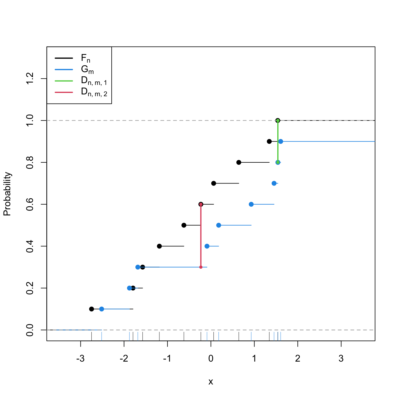

$Kolmogorov–Smirnov distance $D_{n,m}=\max(D_{n,m,1},D_{n,m,2})$ for two samples of sizes $n=m=10$ coming from $F(\cdot)=\Phi\left(\frac{\cdot-\mu_1}{\sigma_1}\right)$ and $G(\cdot)=\Phi\left(\frac{\cdot-\mu_2}{\sigma_2}\right),$ where $\mu_1=\mu_2=0,$ and $\sigma_1=1$ and $\sigma_2=\sqrt{2}.$$

Figure 6.7: Kolmogorov–Smirnov distance $D_{n,m}=\max(D_{n,m,1},D_{n,m,2})$ for two samples of sizes $n=m=10$ coming from $F(\cdot)=\Phi\left(\frac{\cdot-\mu_1}{\sigma_1}\right)$ and $G(\cdot)=\Phi\left(\frac{\cdot-\mu_2}{\sigma_2}\right),$ where $\mu_1=\mu_2=0,$ and $\sigma_1=1$ and $\sigma_2=\sqrt{2}.$

An instance of the use of the ks.test function for the two-sided homogeneity test is given below.

# Check the test for H0 true
set.seed(123456)
x0 <- rgamma(n = 50, shape = 1, scale = 1)
y0 <- rgamma(n = 100, shape = 1, scale = 1)
ks.test(x = x0, y = y0)
## 
##  Exact two-sample Kolmogorov-Smirnov test
## 
## data:  x0 and y0
## D = 0.14, p-value = 0.5185
## alternative hypothesis: two-sided

# Check the test for H0 false
x1 <- rgamma(n = 50, shape = 2, scale = 1)
y1 <- rgamma(n = 75, shape = 1, scale = 1)
ks.test(x = x1, y = y1)
## 
##  Exact two-sample Kolmogorov-Smirnov test
## 
## data:  x1 and y1
## D = 0.35333, p-value = 0.0008513
## alternative hypothesis: two-sided

Two-sample Kolmogorov–Smirnov test (one-sided)

Test purpose. Given $X_1,\ldots,X_n\sim F$ and $Y_1,\ldots,Y_m\sim G,$ it tests $H_0: F=G$ vs. $H_1: F<G.$²³² Rejection of $H_0$ in favor of $H_1$ gives evidence for the local stochastic dominance of $X$ over $Y$ (which may or may not be global).
Statistic definition. The test statistic uses the maximum signed distance between $F_n$ and $G_m$:

\[\begin{align*} D_{n,m}^-:=\sqrt{\frac{nm}{n+m}}\sup_{x\in\mathbb{R}} (G_m(x)-F_n(x)). \end{align*}\]

If $H_1:F<G$ holds, then $D_{n,m}^-$ tends to have large positive values. Conversely, when $H_0:F=G$ or $F>G$ holds, smaller values of $D_{n,m}^-$ are expected, possibly negative. The test rejects $H_0$ when $D_{n,m}^-$ is large.
Statistic computation. The computation of $D_{n,m}^-$ is analogous to that of $D_{n,m}$ given in (6.15), but removing absolute values and changing its sign:²³³

\[\begin{align*} D_{n,m}^-=&\,\max(D_{n,m,1}^-,D_{n,m,2}^-),\\ D_{n,m,1}^-:=&\,\sqrt{\frac{nm}{n+m}}\max_{1\leq i\leq n}\left(G_m(X_{(i)})-\frac{i}{n}\right),\\ D_{n,m,2}^-:=&\,\sqrt{\frac{nm}{n+m}}\max_{1\leq j\leq m}\left(\frac{j}{m}-F_n(Y_{(j)})\right). \end{align*}\]
Distribution under $H_0.$ If $H_0$ holds and $F=G$ is continuous, then $D_{n,m}^-$ has the same asymptotic cdf as $D_{n,m}$.
Highlights and caveats. The one-sided two-sample Kolmogorov–Smirnov test is also distribution-free if $F=G$ is continuous and the samples $X_1,\ldots,X_n$ and $Y_1,\ldots,Y_m$ have no ties.
Implementation in R. For continuous data and continuous $F=G,$ the test statistic $D_{n,m}^-$ and the asymptotic $p$-value are readily available through the ks.test function. The one-sided test is carried out if alternative = "less" or alternative = "greater" (not the defaults). The argument alternative means the direction of cdf dominance: "less" $\equiv F\boldsymbol{<}G;$ "greater" $\equiv F\boldsymbol{>}G.$²³⁴ $\!\!^,$²³⁵ Permutations (see Section 6.2.3) can be used for obtaining non-asymptotic $p$-values and dealing with discrete samples.

# Check the test for H0 true
set.seed(123456)
x0 <- rgamma(n = 50, shape = 1, scale = 1)
y0 <- rgamma(n = 100, shape = 1, scale = 1)
ks.test(x = x0, y = y0, alternative = "less") # H1: F < G
## 
##  Exact two-sample Kolmogorov-Smirnov test
## 
## data:  x0 and y0
## D^- = 0.08, p-value = 0.643
## alternative hypothesis: the CDF of x lies below that of y
ks.test(x = x0, y = y0, alternative = "greater") # H1: F > G
## 
##  Exact two-sample Kolmogorov-Smirnov test
## 
## data:  x0 and y0
## D^+ = 0.14, p-value = 0.2638
## alternative hypothesis: the CDF of x lies above that of y

# Check the test for H0 false
x1 <- rnorm(n = 50, mean = 1, sd = 1)
y1 <- rnorm(n = 75, mean = 0, sd = 1)
ks.test(x = x1, y = y1, alternative = "less") # H1: F < G
## 
##  Exact two-sample Kolmogorov-Smirnov test
## 
## data:  x1 and y1
## D^- = 0.52667, p-value = 2.205e-08
## alternative hypothesis: the CDF of x lies below that of y
ks.test(x = x1, y = y1, alternative = "greater") # H1: F > G
## 
##  Exact two-sample Kolmogorov-Smirnov test
## 
## data:  x1 and y1
## D^+ = 1.4502e-15, p-value = 1
## alternative hypothesis: the CDF of x lies above that of y
# Interpretations:
# 1. Strong rejection of H0: F = G in favor of H1: F < G when
# alternative = "less", as in reality x1 is stochastically greater than y1.
# This outcome allows stating that "there is strong evidence supporting that
# x1 is locally stochastically greater than y1"
# 2. No rejection ("strong acceptance") of H0: F = G versus H1: F > G when
# alternative = "greater". Even if in reality x1 is stochastically greater than
# y1 (so H0 is false), the alternative to which H0 is confronted is even less
# plausible. A p-value ~ 1 indicates one is probably conducting the test in
# the uninteresting direction alternative!

Exercise 6.10 Consider the two populations described in Figure 6.8. $X\sim F$ is not stochastically greater than $Y\sim G.$ However, $Y$ is locally stochastically greater than $X$ in $(-\infty,-0.75).$ Therefore, although hard to detect, the two-sample Kolmogorov–Smirnov test should eventually reject $H_0:F=G$ in favor of $H_1:F>G.$ Conduct a simulation study to verify how fast this rejection takes place:

Simulate $X_1,\ldots,X_n\sim F$ and $Y_1,\ldots,Y_n\sim G.$
Apply ks.test with the corresponding alternative and evaluate if it rejects $H_0$ at significance level $\alpha.$
Repeat Steps 1–2 $M=100$ times and approximate the rejection probability by Monte Carlo.
Perform Steps 1–3 for $n$ taken as seq(10, 3e2, by = 10) and plot the curve of rejection probability as a function of $n.$ Do this for $\alpha=0.10,0.05,0.01.$
Once you have a working solution, increase $M$ to $M=1,000.$ What are your conclusions?
Take now $n$ as seq(50, 3e3, by = 50). Summarize your conclusions.

Two-sample Cramér–von Mises test

Test purpose. Given $X_1,\ldots,X_n\sim F,$ it tests $H_0: F=G$ vs. $H_1: F\neq G$ consistently against all the alternatives in $H_1.$
Statistic definition. The test statistic proposed by Anderson (1962) uses a quadratic distance between $F_n$ and $G_m$:

\[\begin{align} W_{n,m}^2:=\frac{nm}{n+m}\int(F_n(z)-G_m(z))^2\,\mathrm{d}H_{n+m}(z),\tag{6.16} \end{align}\]

where $H_{n+m}$ is the ecdf of the pooled sample $Z_1,\ldots,Z_{n+m},$ where $Z_i:=X_i$ and $Z_{j+n}:=Y_j,$ $i=1,\ldots,n$ and $j=1,\ldots,m.$²³⁶ Therefore, $H_{n+m}(z)=\frac{n}{n+m}F_n(z)+\frac{m}{n+m}G_m(z),$ $z\in\mathbb{R},$ and (6.16) equals²³⁷

\[\begin{align} W_{n,m}^2=\frac{nm}{(n+m)^2}\sum_{k=1}^{n+m}(F_n(Z_k)-G_m(Z_k))^2.\tag{6.17} \end{align}\]
Statistic computation. The formula (6.17) is reasonably direct. Better computational efficiency may be obtained with ranks from the pooled sample.
Distribution under $H_0.$ If $H_0$ holds and $F=G$ is continuous, then $W_{n,m}^2$ has the same asymptotic cdf as $W_n^2$ (see (6.6)).
Highlights and caveats. The two-sample Cramér–von Mises test is also distribution-free if $F_0$ is continuous and the sample has no ties. Otherwise, (6.6) is not the true asymptotic distribution. As in the one-sample case, empirical evidence suggests that the Cramér–von Mises test is often more powerful than the Kolmogorov–Smirnov test. However, the Cramér–von Mises is less versatile, since it does not admit simple modifications to test against one-sided alternatives.
Implementation in R. See below for the statistic implementation. Asymptotic $p$-values can be obtained using goftest::pCvM. Permutations (see Section 6.2.3) can be used for obtaining non-asymptotic $p$-values and dealing with discrete samples.

# Two-sample Cramér-von Mises statistic
cvm2_stat <- function(x, y) {

  # Sample sizes
  n <- length(x)
  m <- length(y)

  # Pooled sample
  z <- c(x, y)

  # Statistic computation via ecdf()
  (n * m / (n + m)^2) * sum((ecdf(x)(z) - ecdf(y)(z))^2)

}

# Check the test for H0 true
set.seed(123456)
x0 <- rgamma(n = 50, shape = 1, scale = 1)
y0 <- rgamma(n = 100, shape = 1, scale = 1)
cvm0 <- cvm2_stat(x = x0, y = y0)
pval0 <- 1 - goftest::pCvM(q = cvm0)
c("statistic" = cvm0, "p-value"= pval0)
## statistic   p-value 
## 0.1294889 0.4585971

# Check the test for H0 false
x1 <- rgamma(n = 50, shape = 2, scale = 1)
y1 <- rgamma(n = 75, shape = 1, scale = 1)
cvm1 <- cvm2_stat(x = x1, y = y1)
pval1 <- 1 - goftest::pCvM(q = cvm1)
c("statistic" = cvm1, "p-value"= pval1)
##    statistic      p-value 
## 1.3283733333 0.0004264598

Two-sample Anderson–Darling test

Test purpose. Given $X_1,\ldots,X_n\sim F,$ it tests $H_0: F=G$ vs. $H_1: F\neq G$ consistently against all the alternatives in $H_1.$
Statistic definition. The test statistic proposed by Pettitt (1976) uses a weighted quadratic distance between $F_n$ and $G_m$:

\[\begin{align} A_{n,m}^2:=\frac{nm}{n+m}\int\frac{(F_n(z)-G_m(z))^2}{H_{n+m}(z)(1-H_{n+m}(z))}\,\mathrm{d}H_{n+m}(z),\tag{6.18} \end{align}\]

where $H_{n+m}$ is the ecdf of $Z_1,\ldots,Z_{n+m}.$ Therefore, (6.18) equals

\[\begin{align} A_{n,m}^2=\frac{nm}{(n+m)^2}\sum_{k=1}^{n+m}\frac{(F_n(Z_k)-G_m(Z_k))^2}{H_{n+m}(Z_k)(1-H_{n+m}(Z_k))}.\tag{6.19} \end{align}\]

In (6.19), it is implicitly assumed that the largest observation of the pooled sample, $Z_{(n+m)},$ is excluded from the sum, since $H_{n+m}(Z_{(n+m)})=1.$²³⁸
Statistic computation. The formula (6.19) is reasonably direct for computation. Better computational efficiency may be obtained with ranks from the pooled sample. The implicit exclusion of $Z_{(n+m)}$ from the sum in (6.19) can be made explicit with

\[\begin{align*} A_{n,m}^2=\frac{nm}{(n+m)^2}\sum_{k=1}^{n+m-1}\frac{(F_n(Z_{(k)})-G_m(Z_{(k)}))^2}{H_{n+m}(Z_{(k)})(1-H_{n+m}(Z_{(k)}))}. \end{align*}\]
Distribution under $H_0.$ If $H_0$ holds and $F=G$ is continuous, then $A_{n,m}^2$ has the same asymptotic cdf as $A_n^2$ (see (6.8)).
Highlights and caveats. The two-sample Anderson–Darling test is also distribution-free if $F_0$ is continuous and the sample has no ties. Otherwise, (6.8) is not the true asymptotic distribution. As in the one-sample case, empirical evidence suggests that the Anderson–Darling test is often more powerful than the Kolmogorov–Smirnov and Cramér–von Mises tests. The two-sample Anderson–Darling test is also less versatile, since it does not admit simple modifications to test against one-sided alternatives.
Implementation in R. See below for the statistic implementation. Asymptotic $p$-values can be obtained using goftest::pAD. Permutations (see Section 6.2.3) can be used for obtaining non-asymptotic $p$-values and dealing with discrete samples.

# Two-sample Anderson-Darling statistic
ad2_stat <- function(x, y) {

  # Sample sizes
  n <- length(x)
  m <- length(y)

  # Pooled sample and pooled ecdf
  z <- c(x, y)
  z <- z[-which.max(z)] # Exclude the largest point
  H <- rank(z) / (n + m)

  # Statistic computation via ecdf()
  (n * m / (n + m)^2) * sum((ecdf(x)(z) - ecdf(y)(z))^2 / ((1 - H) * H))

}

# Check the test for H0 true
set.seed(123456)
x0 <- rgamma(n = 50, shape = 1, scale = 1)
y0 <- rgamma(n = 100, shape = 1, scale = 1)
ad0 <- ad2_stat(x = x0, y = y0)
pval0 <- 1 - goftest::pAD(q = ad0)
c("statistic" = ad0, "p-value"= pval0)
## statistic   p-value 
## 0.8603617 0.4394751

# Check the test for H0 false
x1 <- rgamma(n = 50, shape = 2, scale = 1)
y1 <- rgamma(n = 75, shape = 1, scale = 1)
ad1 <- ad2_stat(x = x1, y = y1)
pval1 <- 1 - goftest::pAD(q = ad1)
c("statistic" = ad1, "p-value"= pval1)
##    statistic      p-value 
## 6.7978295422 0.0004109238

Exercise 6.11 Verify the correctness of the asymptotic null distributions of $W_{n,m}^2$ and $A_{n,m}^2.$ To do so:

Simulate $M=1,000$ pairs of samples of sizes $n=200$ and $m=150$ under $H_0.$
Obtain the statistics $W_{n,m;1}^2,\ldots, W_{n,m;M}^2$ and plot their ecdf.
Overlay the asymptotic cdf of $W_{n,m},$ provided by goftest::pCvM for the one-sample test.
Repeat Steps 2–3 for $A_{n,m}^2.$

Exercise 6.12 Implement in R a single function to properly conduct either the two-sample Cramér–von Mises test or the two-sample Anderson–Darling test. The function must return a tidied "htest" object. Is your implementation of $W_{n,m}^2$ and $A_{n,m}^2$ able to improve cvm2_stat and ad2_stat in speed? Measure the running times for $n=300$ and $m=200$ with the microbenchmark::microbenchmark function.

6.2.2 Specific tests for distribution shifts

Among the previous ecdf-based tests of homogeneity, only the two-sample Kolmogorov–Smirnov test was able to readily deal with one-sided alternatives. However, this test is often more conservative than the Cramér–von Mises and the Anderson–Darling, so it is apparent that there is room for improvement. We next see two nonparametric tests, the Wilcoxon–Mann–Whitney test²³⁹ and the Wilcoxon signed-rank test,²⁴⁰ which are designed to detect one-sided alternatives related to $X$ being stochastically greater than $Y$. Both tests are more powerful than the one-sided Kolmogorov–Smirnov.

In a very vague and imprecise form, these tests can be interpreted as “nonparametric $t$-tests” for unpaired and paired data.²⁴¹ The rationale is that, very often, the aforementioned one-sided alternatives are related to differences in the distributions produced by a shift in their main masses of probability. However, as we will see, there are many subtleties and sides to the previous interpretation. Unfortunately, these nuances are usually ignored in the literature and, as a consequence, the Wilcoxon–Mann–Whitney and Wilcoxon signed-rank tests are massively misunderstood and misused.

Wilcoxon–Mann–Whitney test

The Wilcoxon–Mann–Whitney test addresses the hypothesis testing of

\[\begin{align*} H_0:F=G\quad\text{vs.}\quad H_1:\mathbb{P}[X\geq Y]>0.5. \end{align*}\]

The alternative hypothesis $H_1$ requires special care:

That $\mathbb{P}[X\geq Y]>0.5$ intuitively means that the main mass of probability of $X$ is above that of $Y:$ it is more likely to observe $X\geq Y$ than $X<Y.$
$H_1$ is related to $X$ being stochastically greater than $Y.$ Precisely, $H_1$ is essentially²⁴² implied by the latter:

\[\begin{align*} F(x)<G(x) \text{ for all } x\in\mathbb{R} \implies \mathbb{P}[X\geq Y]\geq 0.5. \end{align*}\]

The converse implication is false (see Figure 6.8). Hence, $H_1:\mathbb{P}[X\geq Y]>0.5$ is more specific than “$X$ is stochastically greater than $Y$”. $H_1$ neither implies nor is implied by the two-sample Kolmogorov–Smirnov’s alternative $H_1':F<G$ (which can be regarded as local stochastic dominance).²⁴³

$Pdfs and cdfs of $X\sim\mathcal{N}(2,4)$ and $Y\sim\mathcal{N}(0,0.25).$ $X$ is not stochastically greater than $Y,$ as the cdfs cross, but $\mathbb{P}\lbrack X\geq Y\rbrack=0.834.$ $Y$ is locally stochastically greater than $X$ in $(-\infty,-0.75).$ The means are shown in vertical lines. Note that the variances of $X$ and $Y$ are not common; recall the difference with respect to the situation in Figure 6.6.$ $Pdfs and cdfs of $X\sim\mathcal{N}(2,4)$ and $Y\sim\mathcal{N}(0,0.25).$ $X$ is not stochastically greater than $Y,$ as the cdfs cross, but $\mathbb{P}\lbrack X\geq Y\rbrack=0.834.$ $Y$ is locally stochastically greater than $X$ in $(-\infty,-0.75).$ The means are shown in vertical lines. Note that the variances of $X$ and $Y$ are not common; recall the difference with respect to the situation in Figure 6.6.$

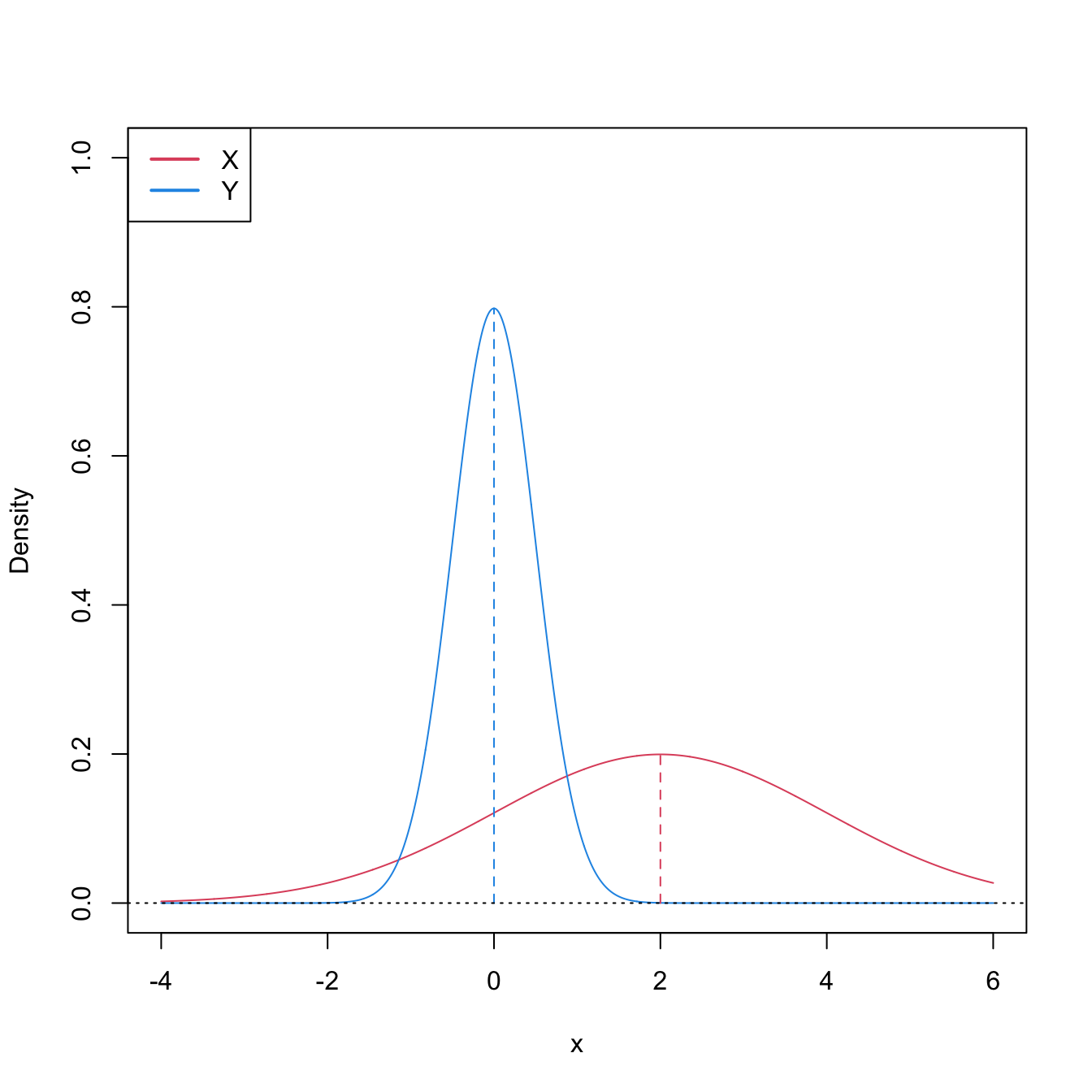
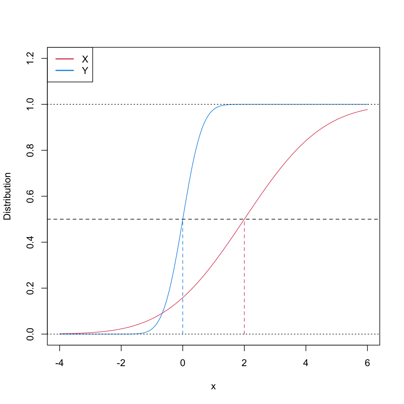
Figure 6.8: Pdfs and cdfs of $X\sim\mathcal{N}(2,4)$ and $Y\sim\mathcal{N}(0,0.25).$ $X$ is not stochastically greater than $Y,$ as the cdfs cross, but $\mathbb{P}\lbrack X\geq Y\rbrack=0.834.$ $Y$ is locally stochastically greater than $X$ in $(-\infty,-0.75).$ The means are shown in vertical lines. Note that the variances of $X$ and $Y$ are not common; recall the difference with respect to the situation in Figure 6.6.

In general, $H_1$ does not directly inform on the medians/means of $X$ and $Y.$ Thus, in general, the Wilcoxon–Mann–Whitney test does not compare medians/means. The probability in $H_1$ is, in general, exogenous to medians/means:²⁴⁴

\[\begin{align} \mathbb{P}[X\geq Y]=\int F_Y(x)\,\mathrm{d}F_X(x).\tag{6.20} \end{align}\]

Only in very specific circumstances $H_1$ is related to medians/means. If $X\sim F$ and $Y\sim G$ are symmetric random variables with medians $m_X$ and $m_Y$ (if the means exist, they equal the medians), then

\[\begin{align} \mathbb{P}[X\geq Y]>0.5 \iff m_X>m_Y.\tag{6.21} \end{align}\]

This characterization informs on the closest the Wilcoxon–Mann–Whitney test gets to a nonparametric version of the $t$-test.²⁴⁵ However, as the two counterexamples in Figures 6.9 and 6.10 respectively illustrate, (6.21) is not true in general, neither for means nor for medians. It may happen that: (i) $\mathbb{P}[X\geq Y]>0.5$ but $\mu_X<\mu_Y;$ or (ii) $\mathbb{P}[X\geq Y]>0.5$ but $m_X<m_Y.$

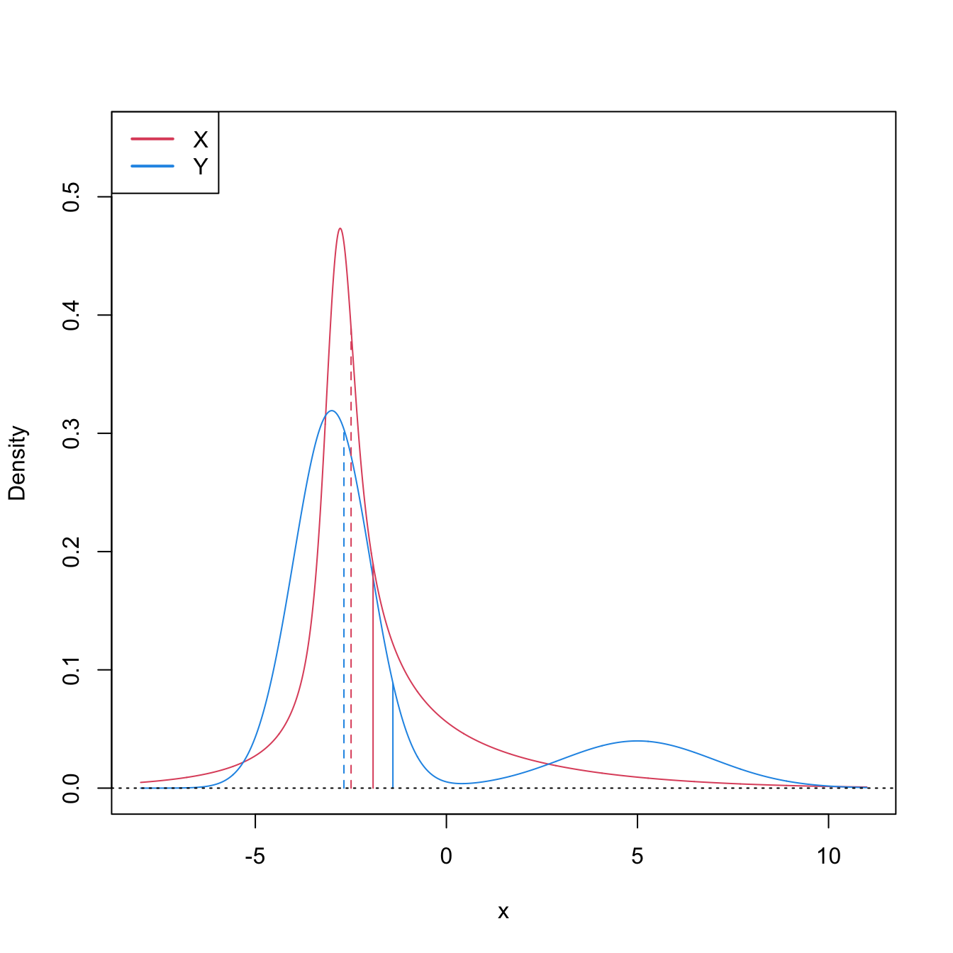
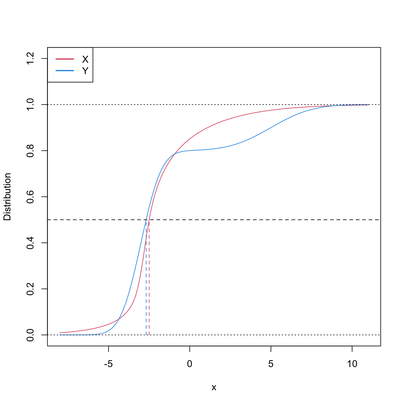
$Pdfs and cdfs of $X$ and $Y\sim0.8\mathcal{N}(-3,1)+0.2\mathcal{N}(5,4),$ where $X$ is distributed as the mixture nor1mix::MW.nm3 but with its standard deviations multiplied by $5$. $\mathbb{P}\lbrack X\geq Y\rbrack=0.5356$ but $\mu_X<\mu_Y,$ since $\mu_X=-1.9189$ and $\mu_Y=-1.4.$ The means are shown in solid vertical lines; the dashed vertical lines stand for the medians $m_X=-2.4944$ and $m_Y=-2.6814.$$ $Pdfs and cdfs of $X$ and $Y\sim0.8\mathcal{N}(-3,1)+0.2\mathcal{N}(5,4),$ where $X$ is distributed as the mixture nor1mix::MW.nm3 but with its standard deviations multiplied by $5$. $\mathbb{P}\lbrack X\geq Y\rbrack=0.5356$ but $\mu_X<\mu_Y,$ since $\mu_X=-1.9189$ and $\mu_Y=-1.4.$ The means are shown in solid vertical lines; the dashed vertical lines stand for the medians $m_X=-2.4944$ and $m_Y=-2.6814.$$

Figure 6.9: Pdfs and cdfs of $X$ and $Y\sim0.8\mathcal{N}(-3,1)+0.2\mathcal{N}(5,4),$ where $X$ is distributed as the mixture nor1mix::MW.nm3 but with its standard deviations multiplied by $5$. $\mathbb{P}\lbrack X\geq Y\rbrack=0.5356$ but $\mu_X<\mu_Y,$ since $\mu_X=-1.9189$ and $\mu_Y=-1.4.$ The means are shown in solid vertical lines; the dashed vertical lines stand for the medians $m_X=-2.4944$ and $m_Y=-2.6814.$

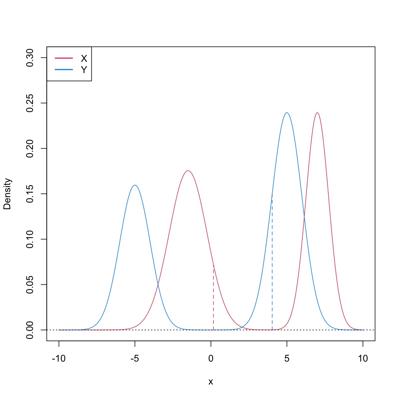
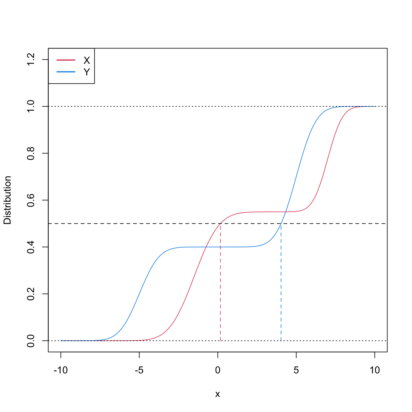
$Pdfs and cdfs of $X\sim0.55\mathcal{N}(-1.5,1.25^2)+0.45\mathcal{N}(7,0.75^2)$ and $Y\sim0.4\mathcal{N}(-5,1)+0.6\mathcal{N}(5,1).$ $\mathbb{P}\lbrack X\geq Y\rbrack=0.6520$ but $m_X<m_Y,$ since $m_X=0.169$ and $m_Y=4.0326.$ The medians are shown in dashed vertical lines; the means are $\mu_X=2.325$ and $\mu_Y=1.$$ $Pdfs and cdfs of $X\sim0.55\mathcal{N}(-1.5,1.25^2)+0.45\mathcal{N}(7,0.75^2)$ and $Y\sim0.4\mathcal{N}(-5,1)+0.6\mathcal{N}(5,1).$ $\mathbb{P}\lbrack X\geq Y\rbrack=0.6520$ but $m_X<m_Y,$ since $m_X=0.169$ and $m_Y=4.0326.$ The medians are shown in dashed vertical lines; the means are $\mu_X=2.325$ and $\mu_Y=1.$$

Figure 6.10: Pdfs and cdfs of $X\sim0.55\mathcal{N}(-1.5,1.25^2)+0.45\mathcal{N}(7,0.75^2)$ and $Y\sim0.4\mathcal{N}(-5,1)+0.6\mathcal{N}(5,1).$ $\mathbb{P}\lbrack X\geq Y\rbrack=0.6520$ but $m_X<m_Y,$ since $m_X=0.169$ and $m_Y=4.0326.$ The medians are shown in dashed vertical lines; the means are $\mu_X=2.325$ and $\mu_Y=1.$

We are now ready to see the main concepts of the Wilcoxon–Mann–Whitney test:

Test purpose. Given $X_1,\ldots,X_n\sim F$ and $Y_1,\ldots,Y_m\sim G,$ it tests $H_0: F=G$ vs. $H_1: \mathbb{P}[X\geq Y]>0.5.$
Statistic definition. On the one hand, the test statistic proposed by Mann and Whitney (1947) directly targets $\mathbb{P}[X\geq Y]$²⁴⁶ with the (unstandardized) estimator

\[\begin{align} U_{n,m;\mathrm{MW}}=\sum_{i=1}^n\sum_{j=1}^m1_{\{X_i>Y_j\}}.\tag{6.22} \end{align}\]

Values of $U_n$ that are significantly larger than $(nm)/2,$ the expected value under $H_0,$ indicate evidence in favor of $H_1.$ On the other hand, the test statistic proposed by Wilcoxon (1945) is

\[\begin{align} U_{n,m;\mathrm{W}}=\sum_{i=1}^n\mathrm{rank}_{X,Y}(Y_i),\tag{6.23} \end{align}\]

where $\mathrm{rank}_{X,Y}(Y_i):=nF_n(Y_i)+mG_m(Y_i)$ is the rank of $Y_i$ on the pooled sample $X_1,\ldots,X_n,Y_1,\ldots,Y_m.$ It happens that the tests based on either (6.22) or (6.23) are equivalent²⁴⁷ when there are no ties on the samples of $X$ and $Y$, since

\[\begin{align} U_{n,m;\mathrm{MW}}=nm+\frac{m(m+1)}{2}-U_{n,m;\mathrm{W}}.\tag{6.24} \end{align}\]
Statistic computation. Computing (6.23) is easier than (6.22).
Distribution under $H_0.$ The test statistic (6.22) is a non-degenerate $U$-statistic. Therefore, since $\mathbb{E}[U_{n,m;\mathrm{MW}}]=(nm)/2$ and $\mathbb{V}\mathrm{ar}[U_{n,m;\mathrm{MW}}]=nm(n+m+1)/12,$ under $H_0$ and with $F=G$ continuous, when $n,m\to\infty,$

\[\begin{align*} \frac{U_{n,m;\mathrm{MW}}-(nm)/2}{\sqrt{nm(n+m+1)/12}}\stackrel{d}{\longrightarrow}\mathcal{N}(0,1). \end{align*}\]
Highlights and caveats. The Wilcoxon–Mann–Whitney test is often regarded as a “nonparametric $t$-test” or as a “nonparametric test for comparing medians”. This interpretation is only correct if both $X$ and $Y$ are symmetric. In this case, it is a nonparametric analogue to the $t$-test. Otherwise, it is a nonparametric extension of the $t$-test that evaluates if there is a shift in the main mass of probability of $X$ or $Y.$ In any case, $H_1:\mathbb{P}[X\geq Y]>0.5$ is related to $X$ being stochastically greater than $Y,$ though it is less strict, and it is not comparable to the one-sided Kolmogorov–Smirnov’s alternative $H_1':F<G.$ The test is distribution-free.
Implementation in R. The test statistic $U_{n,m;\mathrm{MW}}$ (implemented using (6.24)) and the exact/asymptotic $p$-value are readily available through the wilcox.test function. One must specify alternative = "greater" to test $H_0$ against $H_1:\mathbb{P}[X \boldsymbol{\geq}Y]>0.5.$²⁴⁸ The exact cdf of $U_{n,m;\mathrm{MW}}$ under $H_0$ is available in pwilcoxon.

The following code demonstrates how to carry out the Wilcoxon–Mann–Whitney test.

# Check the test for H0 true
set.seed(123456)
n <- 50
m <- 100
x0 <- rgamma(n = n, shape = 1, scale = 1)
y0 <- rgamma(n = m, shape = 1, scale = 1)
wilcox.test(x = x0, y = y0) # H1: P[X >= Y] != 0.5
## 
##  Wilcoxon rank sum test with continuity correction
## 
## data:  x0 and y0
## W = 2403, p-value = 0.7004
## alternative hypothesis: true location shift is not equal to 0
wilcox.test(x = x0, y = y0, alternative = "greater") # H1: P[X >= Y] > 0.5
## 
##  Wilcoxon rank sum test with continuity correction
## 
## data:  x0 and y0
## W = 2403, p-value = 0.6513
## alternative hypothesis: true location shift is greater than 0
wilcox.test(x = x0, y = y0, alternative = "less") # H1: P[X <= Y] > 0.5
## 
##  Wilcoxon rank sum test with continuity correction
## 
## data:  x0 and y0
## W = 2403, p-value = 0.3502
## alternative hypothesis: true location shift is less than 0

# Check the test for H0 false
x1 <- rnorm(n = n, mean = 0, sd = 1)
y1 <- rnorm(n = m, mean = 1, sd = 2)
wilcox.test(x = x1, y = y1) # H1: P[X >= Y] != 0.5
## 
##  Wilcoxon rank sum test with continuity correction
## 
## data:  x1 and y1
## W = 1684, p-value = 0.001149
## alternative hypothesis: true location shift is not equal to 0
wilcox.test(x = x1, y = y1, alternative = "greater") # H1: P[X >= Y] > 0.5
## 
##  Wilcoxon rank sum test with continuity correction
## 
## data:  x1 and y1
## W = 1684, p-value = 0.9994
## alternative hypothesis: true location shift is greater than 0
wilcox.test(x = x1, y = y1, alternative = "less") # H1: P[X <= Y] > 0.5
## 
##  Wilcoxon rank sum test with continuity correction
## 
## data:  x1 and y1
## W = 1684, p-value = 0.0005746
## alternative hypothesis: true location shift is less than 0

# Exact pmf versus asymptotic pdf
# Beware! dwilcox considers (m, n) as the sample sizes of (X, Y)
x <- seq(1500, 3500, by = 100)
plot(x, dwilcox(x = x, m = n, n = m), type = "h", ylab = "Density")
curve(dnorm(x, mean = n * m / 2, sd = sqrt((n * m * (n + m + 1)) / 12)),
      add = TRUE, col = 2)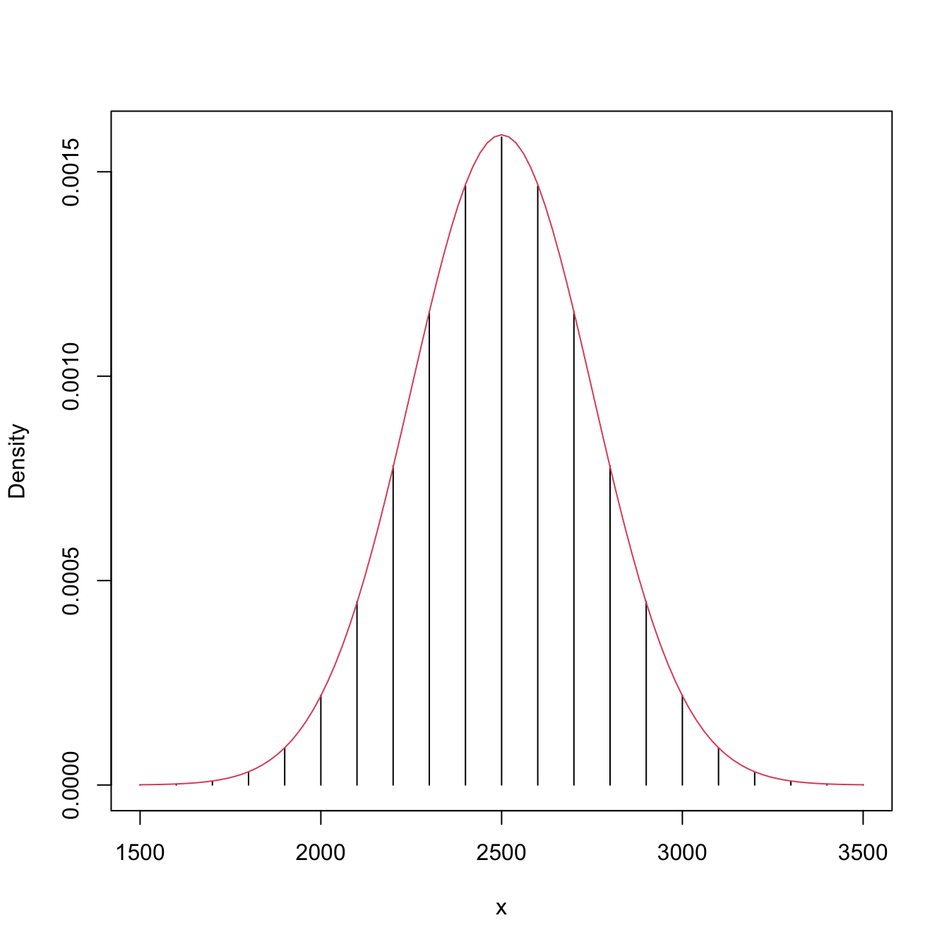

Exercise 6.13 Prove (6.21) for:

Continuous random variables.
Random variables.

Exercise 6.14 Derive (6.20) and, using it, prove that

\[\begin{align*} F_X(x)<F_Y(x)\text{ for all } x\in \mathbb{R}\implies\mathbb{P}[X\geq Y]\geq 0.5. \end{align*}\]

Show that $\mathbb{P}[X\geq Y]>0.5$ is verified if, in addition, $F_X(x)<F_Y(x)$ for $x\in D,$ where $\mathbb{P}[X\in D]>0$ or $\mathbb{P}[Y\in D]>0.$ You can assume $X$ and $Y$ are absolutely continuous variables.

Exercise 6.15 Derive additional counterexamples, significantly different from those in Figures 6.9 and 6.10, for the erroneous claims

$\mu_X>\mu_Y \implies \mathbb{P}[X\geq Y]>0.5;$
$m_X>m_Y \implies \mathbb{P}[X\geq Y]>0.5.$

Exercise 6.16 Verify (6.24) numerically in R with $X$ and $Y$ being continuous random variables. Do so by implementing functions for the test statistics $U_{n,m;\mathrm{MW}}$ and $U_{n,m;\mathrm{W}}$. Check also that (6.24) is not satisfied when the samples of $X$ and $Y$ have ties.

Wilcoxon signed-rank test

Wilcoxon signed-rank test adapts the Wilcoxon–Mann–Whitney test for paired measurements $(X,Y)$ arising from the same individual.

Test purpose. Given $(X_1,Y_1),\ldots,(X_n,Y_n)\sim F,$ it tests $H_0: F_X=F_Y$ vs. $H_1:\mathbb{P}[X\geq Y]>0.5,$ where $F_X$ and $F_Y$ are the marginal cdfs of $X$ and $Y.$
Statistic definition. Wilcoxon (1945)’s test statistic directly targets $\mathbb{P}[X\geq Y],$²⁴⁹ now using the paired observations, with the (unstandardized) estimator

\[\begin{align} S_n:=\sum_{i=1}^n1_{\{X_i>Y_i\}}.\tag{6.25} \end{align}\]

Values of $S_n$ that are significantly larger than $n/2,$ the expected value under $H_0,$ indicate evidence in favor of $H_1.$
Statistic computation. Computing (6.25) is straightforward.
Distribution under $H_0.$ Under $H_0,$ it follows trivially that $S_n\sim\mathrm{B}(n,0.5).$
Highlights and caveats. The Wilcoxon signed-rank test shares the same highlights and caveats as its unpaired counterpart. It can be regarded as a “nonparametric paired $t$-test” if both $X$ and $Y$ are symmetric. In this case, it is a nonparametric analogue to the paired $t$-test. Otherwise, it is a nonparametric extension of the paired $t$-test that evaluates if there is a shift in the main mass of probability of $X$ or $Y$ when both are related.²⁵⁰ The test is distribution-free.
Implementation in R. The test statistic $S_n$ and the exact $p$-value are available through the wilcox.test function. One must specify alternative = "greater" to test $H_0$ against $H_1:\mathbb{P}[X \boldsymbol{\geq}Y]>0.5.$²⁵¹ The exact cdf of $S_n$ under $H_0$ is available in psignrank.

The following code exemplifies how to carry out the Wilcoxon signed-rank test.

# Check the test for H0 true
set.seed(123456)
x0 <- rgamma(n = 50, shape = 1, scale = 1)
y0 <- x0 + rnorm(n = 50)
wilcox.test(x = x0, y = y0, paired = TRUE) # H1: P[X >= Y] != 0.5
## 
##  Wilcoxon signed rank test with continuity correction
## 
## data:  x0 and y0
## V = 537, p-value = 0.3344
## alternative hypothesis: true location shift is not equal to 0
wilcox.test(x = x0, y = y0, paired = TRUE, alternative = "greater")
## 
##  Wilcoxon signed rank test with continuity correction
## 
## data:  x0 and y0
## V = 537, p-value = 0.8352
## alternative hypothesis: true location shift is greater than 0
# H1: P[X >= Y] > 0.5
wilcox.test(x = x0, y = y0, paired = TRUE, alternative = "less")
## 
##  Wilcoxon signed rank test with continuity correction
## 
## data:  x0 and y0
## V = 537, p-value = 0.1672
## alternative hypothesis: true location shift is less than 0
# H1: P[X <= Y] > 0.5

# Check the test for H0 false
x1 <- rnorm(n = 50, mean = 0, sd = 1)
y1 <- x1 + rnorm(n = 50, mean = 1, sd = 2)
wilcox.test(x = x1, y = y1, paired = TRUE) # H1: P[X >= Y] != 0.5
## 
##  Wilcoxon signed rank test with continuity correction
## 
## data:  x1 and y1
## V = 255, p-value = 0.0002264
## alternative hypothesis: true location shift is not equal to 0
wilcox.test(x = x1, y = y1, paired = TRUE, alternative = "greater")
## 
##  Wilcoxon signed rank test with continuity correction
## 
## data:  x1 and y1
## V = 255, p-value = 0.9999
## alternative hypothesis: true location shift is greater than 0
# H1: P[X >= Y] > 0.5
wilcox.test(x = x1, y = y1, paired = TRUE, alternative = "less")
## 
##  Wilcoxon signed rank test with continuity correction
## 
## data:  x1 and y1
## V = 255, p-value = 0.0001132
## alternative hypothesis: true location shift is less than 0
# H1: P[X <= Y] > 0.5

Exercise 6.17 Explore by Monte Carlo the power of the following two-sample tests: one-sided Kolmogorov–Smirnov, Wilcoxon–Mann–Whitney, and $t$-test. Take $\delta=$ 0:3 as the “deviation strength from $H_0$” for the following scenarios:

$X\sim \mathcal{N}(0.25\delta,1)$ and $Y\sim \mathcal{N}(0,1).$
$X\sim t_3+0.25\delta$ and $Y\sim t_1.$
$X\sim 0.5\mathcal{N}(-\delta,(1 + 0.25 \delta)^2)+0.5\mathcal{N}(\delta,(1 + 0.25 \delta)^2)$ and $Y\sim \mathcal{N}(0,2).$

For each scenario, plot the power curves of the three tests for $n=$ seq(10, 200, by = 10). Use $\alpha=0.05.$ Consider first $M=100$ to have a working solution, then increase it to $M=1,000.$ To visualize all the results effectively, you may want to build a Shiny app that, pre-caching the Monte Carlo study, displays the three power curves with respect to $n,$ for a choice of $\delta,$ scenario, and tests to display. Summarize your conclusions in separated points (you may want to visualize first the models a–b).

6.2.3 Permutation-based approach to comparing distributions

Under the null hypothesis of homogeneity, the iid samples $X_1,\ldots,X_n\sim F$ and $Y_1,\ldots,Y_m\sim G$ have the same distributions. Therefore, since both samples are assumed to be independent from each other,²⁵² they are exchangeable under $H_0:F=G$. This means that, for example, the random vector $(X_1,\ldots,X_{\min(n,m)})'$ has the same distribution as $(Y_1,\ldots,Y_{\min(n,m)})'$ under $H_0.$ More generally, each of the $p!$ random subvectors of length $p\leq n+m$ that can be extracted without repetitions from $(X_1,\ldots,X_n,Y_1,\ldots,Y_m)'$ have the exact same distribution under $H_0.$²⁵³ This revelation motivates a resampling procedure that is similar in spirit to the bootstrap seen in Section 6.1.3, yet it is much simpler as it does not require parametric estimation: permutations.

We consider a $N$-permutation function $\sigma:\{1,\ldots,N\}\longrightarrow \{1,\ldots,N\}.$ This function is such that $\sigma(i)=j,$ for certain $i,j\in\{1,\ldots,N\}.$ The number of $N$-permutations quickly becomes extremely large, as there are $N!$ of them.²⁵⁴ As an example, if $N=3,$ there exist $3!=6$ possible $3$-permutations $\sigma_1,\ldots,\sigma_6$:

$i$	$\sigma_1(i)$	$\sigma_2(i)$	$\sigma_3(i)$	$\sigma_4(i)$	$\sigma_5(i)$	$\sigma_6(i)$
$1$	$1$	$1$	$2$	$2$	$3$	$3$
$2$	$2$	$3$	$1$	$3$	$1$	$2$
$3$	$3$	$2$	$3$	$1$	$2$	$1$

Using permutations, it is simple to precise that, for any $(n+m)$-permutation $\sigma,$ under $H_0,$

\[\begin{align} (Z_{\sigma(1)},\ldots,Z_{\sigma(n+m)}) \stackrel{d}{=} (Z_1,\ldots,Z_{n+m}), \tag{6.26} \end{align}\]

where we use the standard notation for the pooled sample, $Z_i=X_i$ and $Z_{j+n}=Y_j$ for $i=1,\ldots,n$ and $j=1,\ldots,m.$ A very important consequence of (6.26) is that, under $H_0,$

\[\begin{align*} T_{n,m}(Z_{\sigma(1)},\ldots,Z_{\sigma(n+m)})\stackrel{d}{=}T_{n,m}(Z_1,\ldots,Z_{n+m}) \end{align*}\]

for any proper test statistic $T_{n,m}$ for $H_0:F=G.$ Therefore, denoting $T_{n,m}\equiv T_{n,m}(Z_1,\ldots,Z_{n+m})$ and $T^{\sigma}_{n,m}\equiv T_{n,m}(Z_{\sigma(1)},\ldots,Z_{\sigma(n+m)}),$ it happens that $\mathbb{P}[T_{n,m}\leq x] = \mathbb{P}[T^\sigma_{n,m}\leq x].$ Hence, it readily follows that

\[\begin{align} \mathbb{P}[T_{n,m}\leq x]=\frac{1}{(n+m)!}\sum_{k=1}^{(n+m)!} \mathbb{P}[T^{\sigma_k}_{n,m}\leq x], \tag{6.27} \end{align}\]

where $\sigma_k$ is the $k$-th out of $(n+m)!$ permutations.

We can now exploit (6.27) to approximate the distribution of $T_{n,m}$ under $H_0.$ The key insight is to realize that, conditionally on the observed sample $Z_1,\ldots,Z_{n+m},$ we know whether or not $T^{\sigma_k}_{n,m}\leq x$ is true. We can then replace $\mathbb{P}[T^{\sigma_k}_{n,m}\leq x]$ with its estimation $1_{\big\{T^{\sigma_k}_{n,m}\leq x\big\}}$ in (6.27). However, the evaluation of the sum of $(n+m)!$ terms is often impossible. Instead, an estimation of its value is obtained by considering $B$ randomly-chosen $(n+m)$-permutations of the pooled sample. Joining these two considerations, it follows that

\[\begin{align} \mathbb{P}[T_{n,m}\leq x]\approx \frac{1}{B}\sum_{b=1}^B 1_{\big\{T^{\hat{\sigma}_b}_{n,m}\leq x\big\}}, \tag{6.28} \end{align}\]

where $\hat{\sigma}_b,$ $b=1,\ldots,B,$ denote the $B$ randomly-chosen $(n+m)$-permutations.²⁵⁵

The null distribution of $T_{n,m}$ can be approximated through (6.28). We summarize next the whole permutation-based procedure for performing a homogeneity test that rejects $H_0$ for large values of the test statistic:

Compute $T_{n,m}\equiv T_{n,m}(Z_1,\ldots,Z_{n+m}).$
Enter the “permutation world”. For $b=1,\ldots,B$:
1. Simulate a randomly-permuted sample $Z_1^{*b},\ldots,Z_{n+m}^{*b}$ from $\{Z_1,\ldots,Z_{n+m}\}.$²⁵⁶
2. Compute $T_{n,m}^{*b}\equiv T_{n,m}(Z_1^{*b},\ldots,Z_{n+m}^{*b}).$
Obtain the $p$-value approximation

\[\begin{align*} p\text{-value}\approx\frac{1}{B}\sum_{b=1}^B 1_{\{T_{n,m}^{*b}> T_{n,m}\}} \end{align*}\]

and emit a test decision from it. Modify it accordingly if rejection of $H_0$ does not happen for large values of $T_{n,m}.$

The following chunk of code provides a template function for implementing the previous algorithm. It is illustrated with an application of the two-sample Anderson–Darling test to discrete data (using the function ad2_stat).

# A homogeneity test using the Anderson-Darling statistic
perm_comp_test <- function(x, y, B = 1e3, plot_boot = TRUE) {

  # Sizes of x and y
  n <- length(x)
  m <- length(y)

  # Test statistic function. Requires TWO arguments, one being the original
  # data (X_1, ..., X_n, Y_1, ..., Y_m) and the other containing the random
  # index for permuting the sample
  Tn <- function(data, perm_index) {

    # Permute sample by perm_index
    data <- data[perm_index]

    # Split into two samples
    x <- data[1:n]
    y <- data[(n + 1):(n + m)]

    # Test statistic -- MODIFY DEPENDING ON THE PROBLEM
    ad2_stat(x = x, y = y)

  }

  # Perform permutation resampling with the aid of boot::boot
  Tn_star <- boot::boot(data = c(x, y), statistic = Tn,
                        sim = "permutation", R = B)

  # Test information -- MODIFY DEPENDING ON THE PROBLEM
  method <- "Permutation-based Anderson-Darling test of homogeneity"
  alternative <- "any alternative to homogeneity"

  # p-value: modify if rejection does not happen for large values of the
  # test statistic
  pvalue <- mean(Tn_star$t > Tn_star$t0)

  # Construct an "htest" result
  result <- list(statistic = c("stat" = Tn_star$t0), p.value = pvalue,
                 statistic_perm = drop(Tn_star$t),
                 B = B, alternative = alternative, method = method,
                 data.name = deparse(substitute(x)))
  class(result) <- "htest"

  # Plot the position of the original statistic with respect to the
  # permutation replicates?
  if (plot_boot) {

    hist(result$statistic_perm, probability = TRUE, 
         main = paste("p-value:", result$p.value), 
         xlab = latex2exp::TeX("$T_{n,m}^*$"))
    rug(result$statistic_perm)
    abline(v = result$statistic, col = 2)

  }

  # Return "htest"
  return(result)

}

# Check the test for H0 true
set.seed(123456)
x0 <- rpois(n = 75, lambda = 5)
y0 <- rpois(n = 75, lambda = 5)
comp0 <- perm_comp_test(x = x0, y = y0, B = 1e3)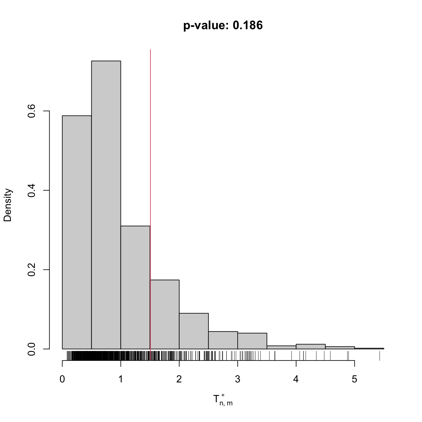

comp0
## 
##  Permutation-based Anderson-Darling test of homogeneity
## 
## data:  x0
## stat = 1.5077, p-value = 0.186
## alternative hypothesis: any alternative to homogeneity

# Check the test for H0 false
x1 <- rpois(n = 50, lambda = 3)
y1 <- rpois(n = 75, lambda = 5)
comp1 <- perm_comp_test(x = x1, y = y1, B = 1e3)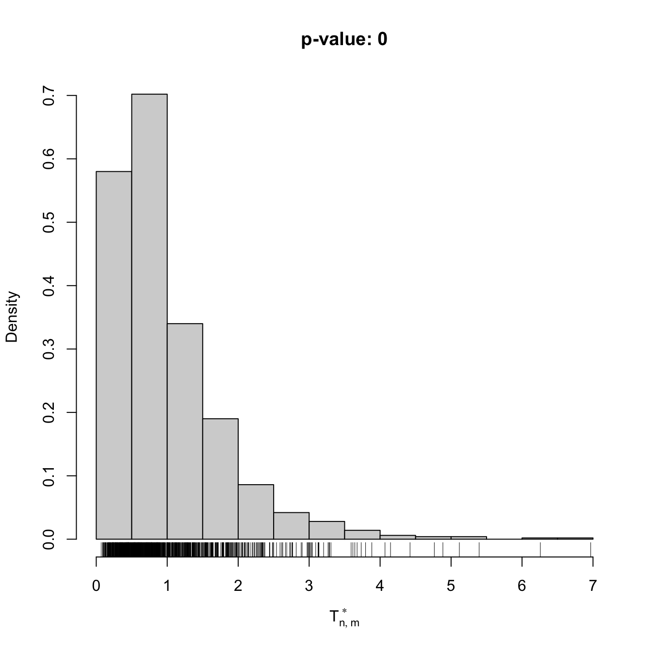

comp1
## 
##  Permutation-based Anderson-Darling test of homogeneity
## 
## data:  x1
## stat = 8.3997, p-value < 2.2e-16
## alternative hypothesis: any alternative to homogeneity

In a paired sample $(X_1,Y_1),\ldots,(X_n,Y_n)\sim F,$ differently to the unpaired case, there is no independence between the $X$- and $Y$-components. Therefore, a variation on the previous permutation algorithm is needed, as the permutation has to be done within the individual observations, and not across individuals. This is achieved by replacing Step i in the previous algorithm with:

Simulate a randomly-permuted sample $(X_1^{*b},Y_1^{*b}),\ldots,(X_n^{*b},Y_n^{*b}),$ where, for each $i=1,\ldots,n,$ $(X_i^{*b},Y_i^{*b})$ is randomly extracted from $\{(X_i,Y_i),(Y_i,X_i)\}.$²⁵⁷

Exercise 6.18 The $F$-statistic $F=\hat{S}^2_1/\hat{S}_2^2$ is employed to test $H_0:\sigma_1^2=\sigma_2^2$ vs. $H_1:\sigma_1^2>\sigma_2^2$ in normal populations $X_1\sim\mathcal{N}(\mu_1,\sigma_1^2)$ and $X_2\sim\mathcal{N}(\mu_2,\sigma_2^2).$ Under $H_0,$ $F$ is distributed as a Snedecor’s $F$ distribution with degrees of freedom $n_1-1$ and $n_2-1.$ The $F$-test is fully parametric. It is implemented in var.test.

The grades.txt dataset contains grades of two exams (e1 and e2) in a certain subject. The group of $41$ students contains two subgroups in mf.

Compute avg, the variable with the average of e1 and e2. Perform a kda of avg for the classes in mf. Then, compare the kde’s of e1 and e2.
Compare the variances of avg for each of the subgroups in mf. Which group has larger sample variance? Perform a permutation-based $F$-test to check if the variance of that group is significantly larger. Compare your results with var.test. Are they coherent?
Compare the variances of e1 and e2. Which exam has larger sample variance? Implement a permutation-based paired $F$-test to assess if there are significant differences in the variances. Do it without relying on boot::boot. Compare your results with the unpaired test from b and with var.test. Are they coherent?

References

Anderson, T. W. 1962. “On the Distribution of the Two-Sample Cramer-von Mises Criterion.” The Annals of Mathematical Statistics 33 (3): 1148–59. https://doi.org/10.1214/aoms/1177704477.

Mann, H. B., and D. R. Whitney. 1947. “On a Test of Whether One of Two Random Variables Is Stochastically Larger Than the Other.” The Annals of Mathematical Statistics 18 (1): 50–60. https://doi.org/10.1214/aoms/1177730491.

Pettitt, A. N. 1976. “A Two-Sample Anderson-Darling Rank Statistic.” Biometrika 63 (1): 161–68. https://doi.org/10.1093/biomet/63.1.161.

Wilcoxon, F. 1945. “Individual Comparisons by Ranking Methods.” Biometrics Bulletin 1 (6): 80–83. https://doi.org/10.2307/3001968.

$F<G$ does not mean that $F(x)<G(x)$ for all $x\in\mathbb{R}.$ If $F(x)>G(x)$ for some $x\in \mathbb{R}$ and $F(x)<G(x)$ or $F(x)=G(x)$ for other $x\in \mathbb{R},$ then $H_1:F<G$ is true!↩︎
Strict because $F(x)<G(x)$ and not $F(x)\leq G(x)$. Since we will use the strict variant of stochastic ordering, we will omit the adjective “strict” henceforth for the sake of simplicity.↩︎
Note that if $F(x)<G(x)$, $\forall x\in\mathbb{R},$ then $X\sim F$ is stochastically greater than $Y\sim G.$ The direction of stochastic dominance is opposite to the direction of dominance of the cdfs.↩︎
With this terminology, clearly global stochastic dominance implies local stochastic dominance, but not the other way around.↩︎
$G_m$ is the ecdf of $Y_1,\ldots,Y_m.$↩︎
Asymptotic when the sample sizes $n$ and $m$ are large: $n,m\to\infty.$↩︎
The case $H_1:F>G$ is analogous and not required, as the roles of $F$ and $G$ can be interchanged.↩︎
Analogously, $D_{n,m,j}^+$ changes the sign inside the maximum of $D_{n,m,j}^-,$ $j=1,2,$ and $D_{n,m}^+:=\max(D_{n,m,1}^+,D_{n,m,2}^+).$↩︎
Confusingly, ks.test’s alternative does not refer to the direction of stochastic dominance, which is the codification used in the alternative arguments of the t.test and wilcox.test functions.↩︎
Observe that ks.test also implements the one-sample Kolmogorov–Smirnov test seen in Section 6.1.1 with one-sided alternatives. That is, one can conduct the test $H_0:F=F_0$ vs. $H_1:F<F_0$ (or $H_1:F>F_0$) using alternative = "less" (or alternative = "greater").↩︎
Observe that $F=G$ is not employed to weight the integrand (6.16), as was the case in (6.4) with $\mathrm{d}F_0(x).$ The reason is because $F=G$ is unknown. However, under $H_0,$ $F=G$ can be estimated better with $H_{n+m}.$↩︎
The Lebesgue–Stieljes integral $\int h(z)\,\mathrm{d}H_{m+n}(z)$ is simply the sum $\frac{1}{n+m}\sum_{k=1}^{n+m} h(Z_k),$ since the pooled ecdf $H_{m+n}$ is a discrete cdf assigning $1/(n+m)$ probability mass to each $Z_k,$ $k=1,\ldots,n+m.$↩︎
Why is the minimum $Z_{(1)}$ not excluded?↩︎
Also known as Wilcoxon rank-sum test, Mann–Whitney $U$ test, and Mann–Whitney–Wilcoxon test. The literature is not unanimous in the terminology, which can be confusing. This ambiguity is partially explained by the almost-coetaneity of the papers by Wilcoxon (1945) and Mann and Whitney (1947).↩︎
Also known as the signed-rank test.↩︎
Recall that the two-sample $t$-test for $H_0:\mu_X=\mu_Y$ vs. $H_1:\mu_X\neq\mu_Y$ (one-sided versions: $H_1:\mu_X>\mu_Y,$ $H_1:\mu_X<\mu_Y$) is actually a nonparametric test for comparing means of arbitrary random variables, possibly non-normal, if employed for large sample sizes. Indeed, due to the CLT, $(\bar{X} -\bar{Y})/\sqrt{(\hat{S}_X^2/n+\hat{S}_Y^2/m)} \stackrel{d}{\longrightarrow}\mathcal{N}(0,1)$ as $n,m\to\infty,$ irrespective of how $X$ and $Y$ are distributed. Here $\hat{S}_X^2$ and $\hat{S}_Y^2$ represent the quasi-variances of $X_1,\ldots,X_n$ and $Y_1,\ldots,Y_m,$ respectively. Equivalently, the one-sample $t$-test for $H_0:\mu_X=\mu_0$ vs. $H_1:\mu_X\neq\mu_0$ (one-sided versions: $H_1:\mu_X>\mu_0,$ $H_1:\mu_X<\mu_0$) is also nonparametric if employed for large sample sizes: $\bar{X}/(\hat{S}/\sqrt{n}) \stackrel{d}{\longrightarrow}\mathcal{N}(0,1)$ as $n\to\infty.$ The function t.test in R implements one/two-sample tests for two/one-sided alternatives.↩︎
Recall the strict inequality in $H_1;$ see Exercise 6.14 for more details.↩︎
Recall that the exact meaning of “$F<G$” was that $F(x)<G(x)$ for some $x\in\mathbb{R},$ not for all $x\in\mathbb{R}.$↩︎
Observe that $\mathbb{P}[Y\geq X]=\int F_X(x)\,\mathrm{d}F_Y(x)$ and how this probability is complementary of (6.20) when $X$ or $Y$ are absolutely continuous.↩︎
Due to the easier interpretation of the Wilcoxon–Mann–Whitney test for symmetric populations, this particular case is sometimes included as an assumption of the test. This simplified presentation of the test unnecessarily narrows its scope.↩︎
Under continuity of $X$ and $Y$.↩︎
Hence the terminology Wilcoxon–Mann–Whitney. Why are the tests based on (6.22) and (6.23) equivalent?↩︎
Observe that wilcox.test also implements the one-sided alternative $H_1:\mathbb{P}[X \boldsymbol{\leq}Y]>0.5$ if alternative = "less" (rejection for small values of (6.22)) and the two equivalent two-sided alternatives $H_1:\mathbb{P}[X \boldsymbol{\geq}Y]\neq 0.5$ or $H_1:\mathbb{P}[X \boldsymbol{\leq}Y]\neq 0.5$ if alternative = "two.sided" (default; rejection for large and small values of (6.22)).↩︎
Again, under continuity.↩︎
Equivalently, it evaluates if the main mass of probability of $X-Y$ is located further from $0.$↩︎
One- and two-sided alternatives are also possible, analogously to the unpaired case.↩︎
We postpone until the end of the section the treatment of the paired sample case.↩︎
If repetitions were allowed, the distributions would be degenerate. For example, if $X_1,X_2,X_3$ are iid, the distribution of $(X_1,X_1,X_2)$ is degenerate.↩︎
If $N=60,$ there are $8.32\times 10^{81}$ $N$-permutations. This number is already $10$ times larger than the estimated number of atoms in the observable universe.↩︎
Since $N!=(n+m)!$ quickly becomes extremely large, the probability of obtaining at least one duplicated permutation among $B$ randomly-extracted permutations (with replacement) is very small. Precisely, the probability is pbirthday(n = B, classes = factorial(N)). If $B=10^4$ and $N=18!$ ($n=m=9$), this probability is $7.81\times 10^{-9}.$↩︎
This sampling is done by extracting, without replacement, elements from the pooled sample z <- c(x, y). This can be simply done with sample(z).↩︎
This sampling is done by switching, randomly for each row, the columns of the sample. If z <- cbind(x, y), this can be simply done with ind_perm <- runif(n) > 0.5; z[ind_perm, ] <- z[ind_perm, 2:1].↩︎

\(i\)	\(\sigma_1(i)\)	\(\sigma_2(i)\)	\(\sigma_3(i)\)	\(\sigma_4(i)\)	\(\sigma_5(i)\)	\(\sigma_6(i)\)
\(1\)	\(1\)	\(1\)	\(2\)	\(2\)	\(3\)	\(3\)
\(2\)	\(2\)	\(3\)	\(1\)	\(3\)	\(1\)	\(2\)
\(3\)	\(3\)	\(2\)	\(3\)	\(1\)	\(2\)	\(1\)