2.2 Kernel density estimation

The moving histogram (2.3) can be equivalently written as

\[\begin{align} \hat{f}_\mathrm{N}(x;h)&=\frac{1}{2nh}\sum_{i=1}^n1_{\{x-h<X_i<x+h\}}\nonumber\\ &=\frac{1}{nh}\sum_{i=1}^n\frac{1}{2}1_{\left\{-1<\frac{x-X_i}{h}<1\right\}}\nonumber\\ &=\frac{1}{nh}\sum_{i=1}^nK\left(\frac{x-X_i}{h}\right), \tag{2.6} \end{align}\]

with $K(z)=\frac{1}{2}1_{\{-1<z<1\}}.$ Interestingly, $K$ is a uniform density in $(-1,1)$! This means that, when approximating

\[\begin{align*} \mathbb{P}[x-h<X<x+h]=\mathbb{P}\left[-1<\frac{x-X}{h}<1\right] \end{align*}\]

by (2.6), we are giving equal weight to all the points $X_1,\ldots,X_n.$ The generalization of (2.6) to non-uniform weighting is now obvious: replace $K$ with an arbitrary density! Then $K$ is known as a kernel. As it is commonly²¹ assumed, we consider $K$ to be a density that is symmetric and unimodal at zero. This generalization provides the definition of the kernel density estimator (kde)²²:

\[\begin{align} \hat{f}(x;h):=\frac{1}{nh}\sum_{i=1}^nK\left(\frac{x-X_i}{h}\right). \tag{2.7} \end{align}\]

A common notation is $K_h(z):=\frac{1}{h}K\left(\frac{z}{h}\right),$ the so-called scaled kernel, so that the kde is written as $\hat{f}(x;h)=\frac{1}{n}\sum_{i=1}^nK_h(x-X_i).$

Figure 2.6: Construction of the kernel density estimator. The animation shows how bandwidth and kernel affect the density estimate, and how the kernels are rescaled densities with modes at the data points. Application available here.

It is useful to recall (2.7) with the normal kernel. If that is the case, then $K_h(x-X_i)=\phi_h(x-X_i)$ and the kernel is the density of a $\mathcal{N}(X_i,h^2).$ Thus the bandwidth $h$ can be thought of as the standard deviation of a normal density with mean $X_i,$ and the kde (2.7) as a data-driven mixture of those densities. Figure 2.6 illustrates the construction of the kde and the bandwidth and kernel effects.

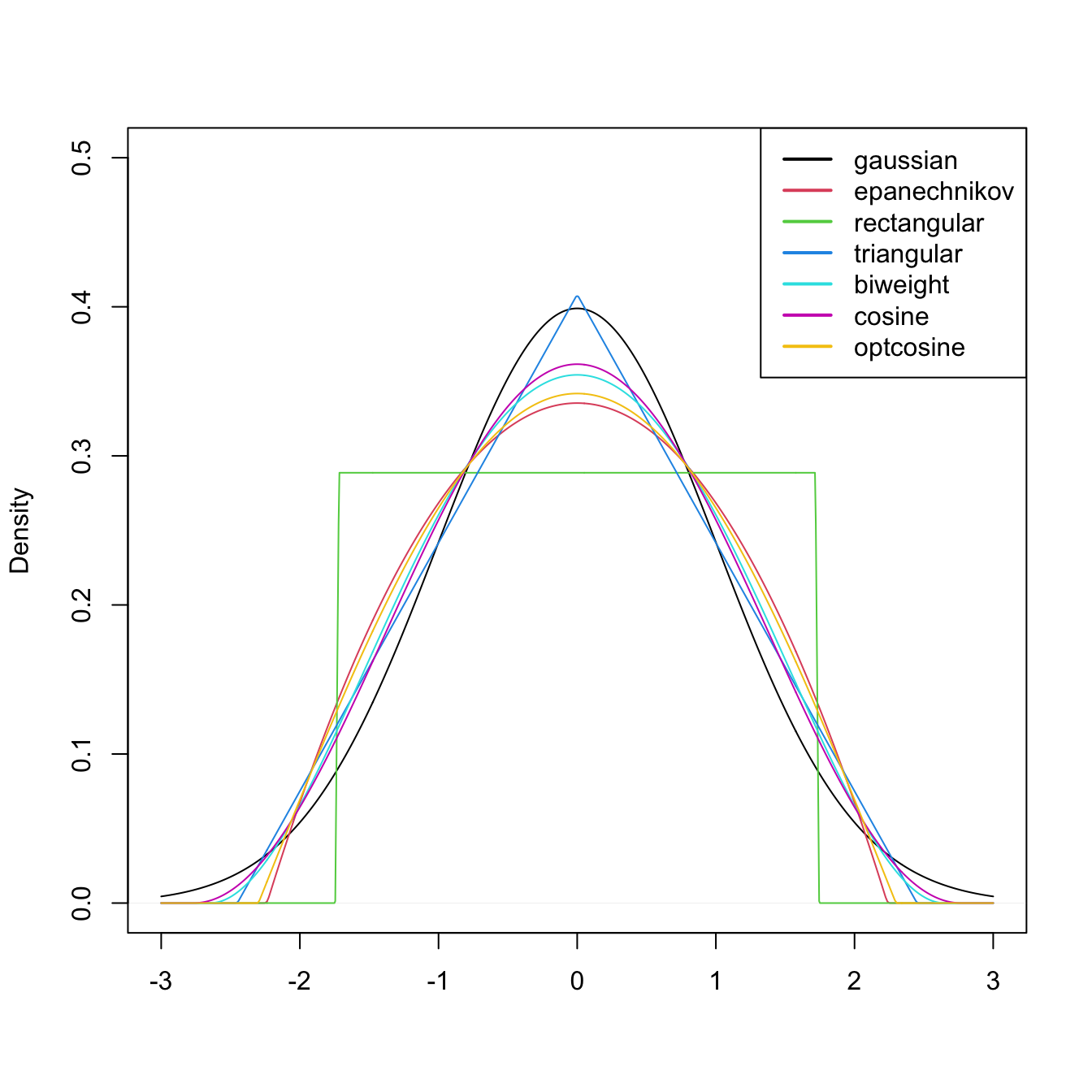
Figure 2.7: Several scaled kernels from R’s density function. See (2.9) in the remark below for the different parametrization.

Several types of kernels are possible. Figure 2.7 illustrates the form of several implemented in R’s density function. The most popular is the normal kernel $K(z)=\phi(z),$ although the Epanechnikov kernel, $K(z)=\frac{3}{4}(1-z^2)1_{\{|z|<1\}},$ is the most efficient.²³ The rectangular kernel $K(z)=\frac{1}{2}1_{\{|z|<1\}}$ yields the moving histogram as a particular case. Importantly, the kde inherits the smoothness properties of the kernel. That means, for example, that (2.7) with a normal kernel is infinitely differentiable. But with an Epanechnikov kernel, (2.7) is not differentiable, and with a rectangular kernel is not even continuous. However, if a certain smoothness is guaranteed (continuity at least), the choice of the kernel has little importance in practice, at least in comparison with the much critical choice of the bandwidth $h.$

The computation of the kde in R is done through the density function. The function automatically chooses the bandwidth $h$ using a data-driven criterion²⁴ referred to as a bandwidth selector. Bandwidth selectors will be studied in detail in Section 2.4.

# Sample 100 points from a N(0, 1)
set.seed(1234567)
samp <- rnorm(n = 100, mean = 0, sd = 1)

# Quickly compute a kde and plot the density object
# Automatically chooses bandwidth and uses normal kernel
plot(density(x = samp))

# Select a particular bandwidth (0.5) and kernel (Epanechnikov)
lines(density(x = samp, bw = 0.5, kernel = "epanechnikov"), col = 2)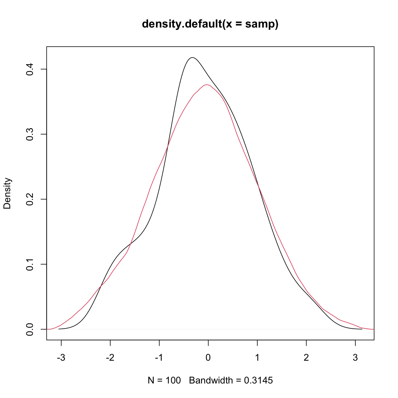


# density() automatically chooses the interval for plotting the kde
# (observe that the black line goes to roughly between -3 and 3)
# This can be tuned using "from" and "to"
plot(density(x = samp, from = -4, to = 4), xlim = c(-5, 5))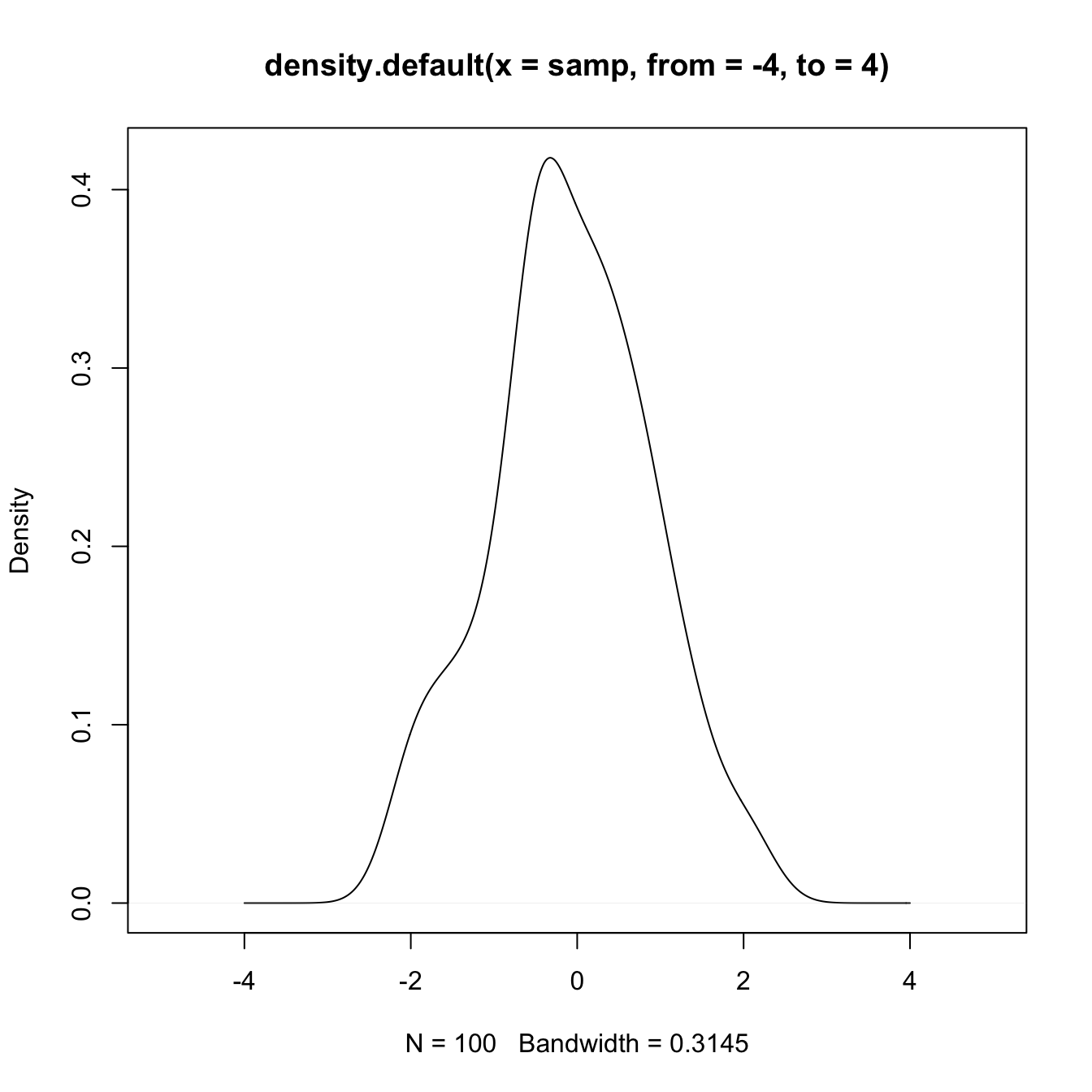


# The density object is a list
kde <- density(x = samp, from = -5, to = 5, n = 1024)
str(kde)
## List of 7
##  $ x        : num [1:1024] -5 -4.99 -4.98 -4.97 -4.96 ...
##  $ y        : num [1:1024] 4.91e-17 2.97e-17 1.86e-17 2.53e-17 3.43e-17 ...
##  $ bw       : num 0.315
##  $ n        : int 100
##  $ call     : language density.default(x = samp, n = 1024, from = -5, to = 5)
##  $ data.name: chr "samp"
##  $ has.na   : logi FALSE
##  - attr(*, "class")= chr "density"
# Note that the evaluation grid "x" is not directly controlled, only through
# "from, "to", and "n" (better use powers of 2)
plot(kde$x, kde$y, type = "l")
curve(dnorm(x), col = 2, add = TRUE) # True density
rug(samp)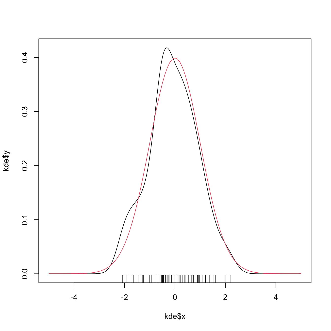

Exercise 2.6 Employing the normal kernel:

Estimate and plot the density of faithful$eruptions.
Create a new plot and superimpose different density estimations with bandwidths equal to $0.1,$ $0.5,$ and $1.$
Get the density estimate at exactly the point $x=3.1$ using $h=0.15.$

We next introduce an important remark about the use of the density function. Before that, we need some notation. From now on, we consider the integrals to be over $\mathbb{R}$ if not stated otherwise. In addition, we denote

\[\begin{align*} \mu_2(K):=\int z^2 K(z)\,\mathrm{d}z \end{align*}\]

to the second-order moment²⁵ of $K.$

Remark. The kernel, say $\tilde K,$ employed in density uses a parametrization that guarantees that $\mu_2(\tilde K)=1.$ This implies that the variance of the scaled kernel is $h^2,$ that is, that $\mu_2(\tilde K_h)=h^2.$ These normalized kernels may be different from the ones we have considered in the exposition. For example, the uniform kernel $K(z)=\frac{1}{2}1_{\{-1<z<1\}},$ for which $\mu_2(K)=\frac{1}{3},$ is implemented in R as $\tilde K(z)=\frac{1}{2\sqrt{3}}1_{\{-\sqrt{3}<z<\sqrt{3}\}}$ (observe in Figure 2.7 that the rectangular kernel takes the value $\frac{1}{2\sqrt{3}}\approx 0.29$).

The density’s normalized kernel $\tilde K$ can be obtained from $K,$ and vice versa, with a straightforward derivation. On the one hand, since $\mu_2(K) = \int z^2 K(z),$

\[\begin{align} 1 &= \int \frac{z^2}{\mu_2(K)} K(z)\,\mathrm{d}z\nonumber\\ &= \int t^2 K\left(\mu_2(K)^{1/2} t\right)\mu_2(K)^{1/2}\,\mathrm{d}t\tag{2.8} \end{align}\]

by making the change of variables $t=\frac{z}{\mu_2(K)^{1/2}}$ in the second equality. Now, based on (2.8), define

\[\begin{align} \tilde K(z) := \mu_2(K)^{1/2}K\left(\mu_2(K)^{1/2} z\right) \tag{2.9} \end{align}\]

and this is a kernel that satisfies $\mu_2(\tilde K)=\int t^2 \tilde K(t)\,\mathrm{d}t = 1$ and is a density unimodal about $0.$ It is indeed the kernel employed by density.

Therefore, if we consider a bandwidth $h$ for the normalized kernel $\tilde K$ (resulting $\tilde K_h$), we have that

\[\begin{align*} \tilde K_h(z) = \frac{\mu_2(K)^{1/2}}{h} K\left(\frac{\mu_2(K)^{1/2}z}{h}\right) = K_{\tilde h}(z) \end{align*}\]

where

\[\begin{align} \tilde h := \mu_2(K)^{-1/2}h. \end{align}\]

As a consequence, a normalized kernel $\tilde K$ with a given bandwidth $h$ (for example, the one considered in density’s bw) has an associated scaled bandwidth $\tilde h$ for the unnormalized kernel $K.$

The following code numerically illustrates the difference between $\tilde K$ and $K$ for the Epanechnikov kernel.

# Implementation of the Epanechnikov based on the theory
K_Epa <- function(z, h = 1) 3 / (4 * h) * (1 - (z / h)^2) * (abs(z) < h)
mu2_K_Epa <- integrate(function(z) z^2 * K_Epa(z), lower = -1, upper = 1)$value

# Epanechnikov kernel by R
h <- 0.5
plot(density(0, kernel = "epanechnikov", bw = h))

# Build the equivalent bandwidth
h_tilde <- h / sqrt(mu2_K_Epa)
curve(K_Epa(x, h = h_tilde), add = TRUE, col = 2)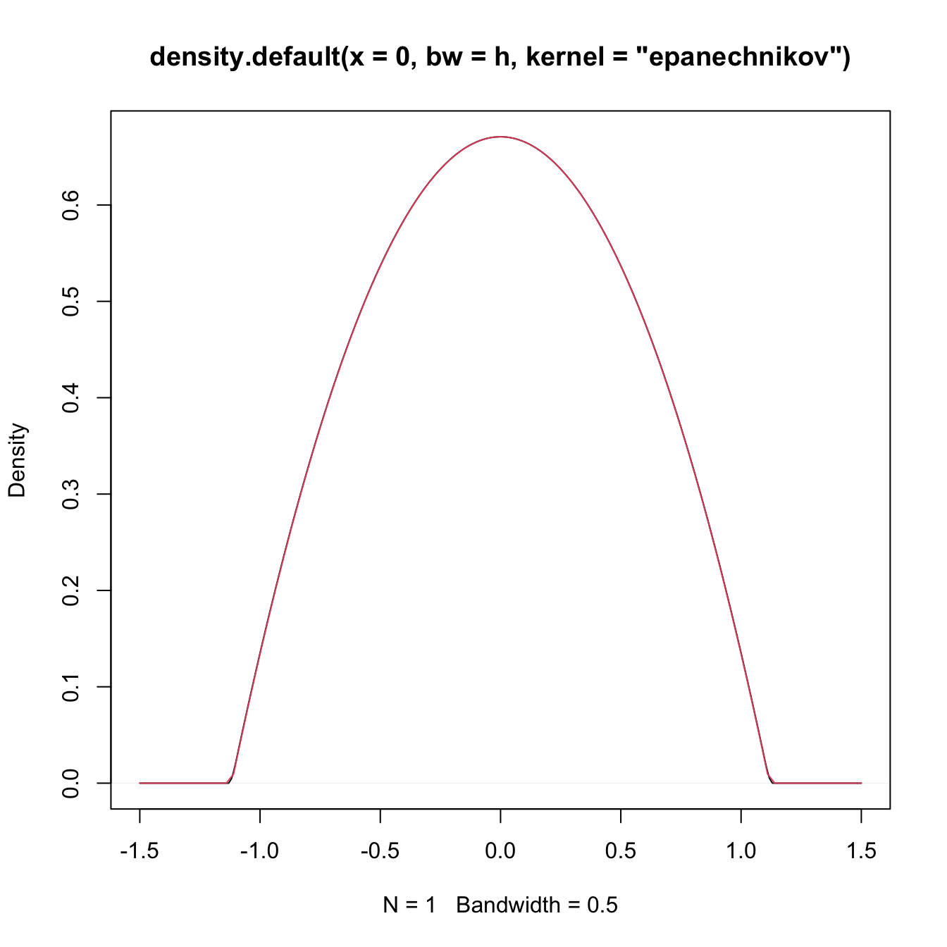


# The other way around
h_tilde <- 2
h <- h_tilde * sqrt(mu2_K_Epa)
curve(K_Epa(x, h = h_tilde), from = -3, to = 3, col = 2)
lines(density(0, kernel = "epanechnikov", bw = h))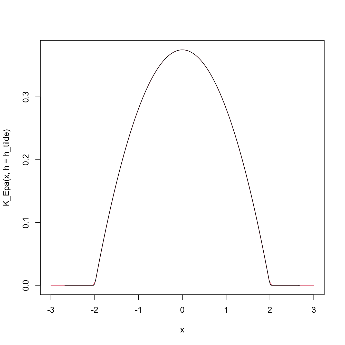

Exercise 2.7 Obtain the kernel $\tilde K$ for:

the normal kernel $K(z)=\phi(z);$
the Epanechnikov kernel $K(z)=\frac{3}{4}(1-z^2)1_{\{|z|<1\}};$
the kernel $K(z)=(1-|z|)1_{\{|z|<1\}}.$

Exercise 2.8 Given $h,$ obtain $\tilde h$ such that $\tilde K_h = K_{\tilde h}$ for:

the uniform kernel $K(z)=\frac{1}{2}1_{\{|z|<1\}};$
the kernel $K(z)=\frac{1}{2\pi}(1+\cos(z))1_{\{|z|<\pi\}};$
the kernel $K(z)=(1-|z|)1_{\{|z|<1\}}.$

Exercise 2.9 Repeat Exercise 2.6, but now considering the Epanechnikov kernel in its unnormalized form. To do so, find the adequate bandwidths to input in density’s bw.

References

Parzen, E. 1962. “On Estimation of a Probability Density Function and Mode.” Annals of Mathematical Statistics 33 (3): 1065–76. https://doi.org/10.1214/aoms/1177704472.

Rosenblatt, M. 1956. “Remarks on Some Nonparametric Estimates of a Density Function.” Annals of Mathematical Statistics 27 (3): 832–37. https://doi.org/10.1214/aoms/1177728190.

In greater generality, the kernel $K$ might only be assumed to be an integrable function with unit integral.↩︎
Also known as the Parzen–Rosemblatt estimator to honor the proposals by Parzen (1962) and Rosenblatt (1956).↩︎
Although the efficiency of the normal kernel, with respect to the Epanechnikov kernel, is roughly $0.95.$↩︎
Precisely, the rule-of-thumb given by bw.nrd.↩︎
The variance, since $\int zK(z)\,\mathrm{d}z=0$ because the kernel is symmetric with respect to zero.↩︎