3.5 Applications of kernel density estimation

Once we are able to adequately estimate the multivariate density $f$ of a random vector $\mathbf{X}$ by $\hat{f}(\cdot;\mathbf{H}),$ we can perform a series of interesting applications that go beyond the mere visualization and graphical description of the estimated density. These applications are intimately related to multivariate analysis methods rooted on the normality assumption:

Density level set estimation. The level set of the density $f$ at level $c\geq0$ is defined as $\mathcal{L}(f;c):=\{\mathbf{x}\in\mathbb{R}^p: f(\mathbf{x})\geq c\}.$ An estimation of $\mathcal{L}(f;c)$ is useful to visualize the highest density regions, which give a concise view of the most likely values for $\mathbf{X}$ and therefore summarize the structure of $\mathbf{X}.$ In addition, this summary is produced without needing to restrict to connected sets,⁷³ as the box plot⁷⁴ does,⁷⁵ and with the additional benefit of determining the approximate probability contained in them. Level sets also are useful to estimate the support of $\mathbf{X}$ and to detect multivariate outliers without the need to employ the Mahalanobis distance.⁷⁶
Clustering or unsupervised learning. The aim of clustering techniques, such as hierarchical clustering or $k$-means,⁷⁷ is to find homogeneous clusters (subgroups) within the sample (group). Despite their usefulness, these two techniques have important drawbacks: they do not automatically determine the number of clusters and they lack a simple interpretation in terms of the population, relying entirely on the sample for its construction and performance evaluation. Based on a density $f,$ the population clusters of the domain of $\mathbf{X}$ can be precisely defined as the “domains of attraction of the density modes”. The mean shift clustering algorithm replaces $f$ with $\hat{f}(\cdot;\mathbf{H})$ and gives a neat clustering recipe that automatically determines the number of clusters.
Classification or supervised learning. Suppose $\mathbf{X}$ has a categorical random variable $Y$ as a companion, the labels of which indicate several classes within the population $\mathbf{X}.$ Then, the task of assigning a point $\mathbf{x}\in\mathbb{R}^p$ to a class of $Y,$ based on a sample $(\mathbf{X}_1,Y_1),\ldots,(\mathbf{X}_n,Y_n),$ is a classification problem. Classic multivariate techniques such as Linear Discriminant Analysis (LDA) and Quadratic Discriminant Analysis (QDA)⁷⁸ tackle this task by confronting normals associated with each class, say $\mathcal{N}_p(\boldsymbol{\mu}_1,\boldsymbol{\Sigma}_1)$ and $\mathcal{N}_p(\boldsymbol{\mu}_2,\boldsymbol{\Sigma}_2),$ and then assigning $\mathbf{x}\in\mathbb{R}^p$ to the class that maximizes $\phi_{\hat{\boldsymbol{\Sigma}}_i}(\mathbf{x}-\hat{\boldsymbol{\mu}}_i),$ $i=1,2.$ The very same principle can be followed by replacing the estimated normal densities with the kdes of each class.
Description of the main features of the data. Principal Component Analysis (PCA) is a very well-known linear dimension-reduction technique that is closely related to the normal distribution.⁷⁹ PCA helps to describe the main features of a dataset by estimating the principal directions on $\mathbb{R}^p,$ $p\geq2,$ of the maximum projected variance of $\mathbf{X}.$ These principal directions are highly related to the density ridges of $\phi_{\boldsymbol{\Sigma}}(\cdot-\boldsymbol{\mu}),$ the latter concept generating flexible principal curves for any density $f.$ As a consequence, density ridges of $\hat{f}(\cdot;\mathbf{H})$ give a flexible nonlinear description of the structure of the data.

Next, we review the details associated with these applications, which are excellently described in Chapters 6 and 7 in Chacón and Duong (2018).

3.5.1 Level set estimation

The estimation of the level set $\mathcal{L}(f;c)=\{\mathbf{x}\in\mathbb{R}^p: f(\mathbf{x})\geq c\},$ useful to determine high-density regions, can be straightforwardly done by plugging the kde of $f$ and considering

\[\begin{align*} \mathcal{L}(\hat{f}(\cdot;\mathbf{H});c) = \{\mathbf{x}\in\mathbb{R}^p:\hat{f}(\mathbf{x};\mathbf{H})\geq c\}. \end{align*}\]

Obtaining the representation of $\mathcal{L}(\hat{f}(\cdot;\mathbf{H});c)$ in practice involves considering a grid in $\mathbb{R}^p$ in order to evaluate the condition $\hat{f}(\mathbf{x};\mathbf{H})\geq c$ and to determine the region of $\mathbb{R}^p$ in which it is satisfied.

We illustrate the computation of $\mathcal{L}(\hat{f}(\cdot;\mathbf{H});c)$ for a couple of simulated examples in $\mathbb{R}.$ Notice, in the code below, how the function kde_level_set automatically deals with the annoyance that $\mathcal{L}(\hat{f}(\cdot;\mathbf{H});c)$ may not be a connected region, that is, that $\mathcal{L}(\hat{f}(\cdot;\mathbf{H});c)=\bigcup_{i=1}^k[a_i,b_i]$ with $k$ unknown beforehand.

# Simulated sample
n <- 100
set.seed(12345)
samp <- rnorm(n = n)

# Kde as usual, but force to evaluate it at seq(-4, 4, length = 4096)
bw <- bw.nrd(x = samp)
kde <- density(x = samp, bw = bw, n = 4096, from = -4, to = 4)

# For a given c, what is the theoretical level set? Since we know that the
# real density is symmetric and unimodal, then the level set is an interval
# of the form [-x_c, x_c]
c <- 0.2
x_c <- tryCatch(uniroot(function(x) dnorm(x) - c, lower = 0, upper = 4)$root,
                error = function(e) NA)

# Show theoretical level set
x <- seq(-4, 4, by = 0.01)
plot(x, dnorm(x), type = "l", ylim = c(0, 0.5), ylab = "Density")
rug(samp)
polygon(x = c(-x_c, -x_c, x_c, x_c), y = c(0, c, c, 0),
        col = rgb(0, 0, 0, alpha = 0.5), density = 10)

# Function to compute and plot a kde level set. Observe that kde stands for an
# object containing the output of density(), although obvious modifications
# could be done to the function to receive a ks::kde object
# as the main argument
kde_level_set <- function(kde, c, add_plot = FALSE, ...) {

  # Begin and end index for the potentially many intervals in the level sets
  # of the kde
  kde_larger_c <- kde$y >= c
  run_length_kde <- rle(kde_larger_c) # Trick to compute the length of the
  # sequence of TRUEs that indicates an interval for which kde$y >= c
  begin <- which(diff(kde_larger_c) > 0) + 1 # Trick to search for the beginning
  # of each of the intervals
  end <- begin + run_length_kde$lengths[run_length_kde$values] - 1 # Compute
  # the end of the intervals from begin + length

  # Add polygons to a density plot? If so, ... are the additional parameters
  # for polygon()
  if (add_plot) {

    apply(cbind(begin, end), 1, function(ind) {
      polygon(x = c(kde$x[ind[1]], kde$x[ind[1]],
                    kde$x[ind[2]], kde$x[ind[2]]),
              y = c(0, kde$y[ind[1]],
                    kde$y[ind[2]], 0), ...)
      })

  }

  # Return the [a_i, b_i], i = 1, ..., K in the K rows
  return(cbind(kde$x[begin], kde$x[end]))

}

# Add kde and level set
lines(kde, col = 2)
kde_level_set(kde = kde, c = c, add_plot = TRUE,
              col = rgb(1, 0, 0, alpha = 0.5))
##          [,1]     [,2]
## [1,] -1.01685 1.444689
abline(h = c, col = 4) # Level
legend("topright", legend = c("True density", "Kde", "True level set",
                              "Kde level set", "Level c"),
       lwd = 2, col = c(1, 2, rgb(0:1, 0, 0, alpha = 0.5), 4))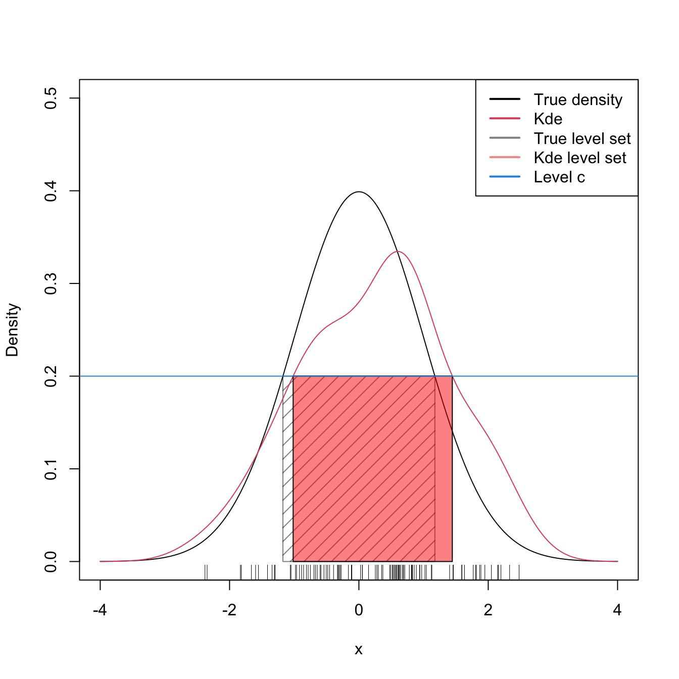

$Level set $\mathcal{L}(f;c)$ and its estimation by $\mathcal{L}(\hat{f}(\cdot;h);c)$ for $c=0.2$ and $f=\phi.$$

Figure 3.4: Level set $\mathcal{L}(f;c)$ and its estimation by $\mathcal{L}(\hat{f}(\cdot;h);c)$ for $c=0.2$ and $f=\phi.$

The following code chunk illustrates how changing the bandwidth $h$ and the level of the set $c$ affects the connectedness of $\mathcal{L}(\hat{f}(\cdot;h);c).$

# Simulated sample
n <- 100
set.seed(12345)
samp <- rnorm(n = n)

# Interactive visualization
x <- seq(-4, 4, by = 0.01)
manipulate::manipulate({

  # Show theoretical level set
  plot(x, dnorm(x), type = "l", ylim = c(0, 0.5), ylab = "Density")
  rug(samp)
  x_c <- tryCatch(uniroot(function(x) dnorm(x) - c, lower = 0, upper = 4)$root,
                  error = function(e) NA) # tryCatch() to bypass errors
  polygon(x = c(-x_c, -x_c, x_c, x_c), y = c(0, c, c, 0),
          col = rgb(0, 0, 0, alpha = 0.5), density = 10)

  # Add estimation
  kde <- density(x = samp, bw = bw, n = 1e5, from = -4, to = 4)
  lines(kde, col = 2)
  kde_level_set(kde = kde, c = c, add_plot = TRUE,
                col = rgb(1, 0, 0, alpha = 0.5))
  abline(h = c, col = 4) # Level
  legend("topright", legend = c("True density", "Kde", "True level set",
                                "Kde level set", "Level c"),
         lwd = 2, col = c(1, 2, rgb(0:1, 0, 0, alpha = 0.5), 4))

}, c = manipulate::slider(min = 0.01, max = 0.5, initial = 0.2, step = 0.01),
bw = manipulate::slider(min = 0.01, max = 1, initial = 0.25, step = 0.01))

Exercise 3.12 Consider the bimodal density $f$ given in nor1mix::MW.nm6. Consider $c=0.15,0.25.$

Compute $\mathcal{L}(f;c).$
From a sample of size $n=200,$ compute $\mathcal{L}(\hat{f}(\cdot;\hat{h}_\mathrm{DPI});c).$

Highest density regions for a given probability

The level $c$ in $\mathcal{L}(f;c)=\{\mathbf{x}\in\mathbb{R}^p: f(\mathbf{x})\geq c\}$ may be difficult to interpret: its effective scale depends on the dimension⁸⁰ $p$ of the random vector $\mathbf{X}$ and on the units in which their components are measured. A more convenient parametrization of the level set is attained if we state the probability that is intended to contain, rather than the minimum value of the density attained in the region. For that purpose, it is usually considered the largest⁸¹ $c_\alpha$ such that

\[\begin{align*} \int_{\mathcal{L}(f;c_\alpha)}f(\mathbf{x})\,\mathrm{d}\mathbf{x}\geq 1-\alpha, \quad \alpha\in(0,1). \end{align*}\]

This formulation raises a key interpretation of $\mathcal{L}(f;c_\alpha)$:

$\mathcal{L}(f;c_\alpha)$ is the smallest⁸² region of $\mathbb{R}^p$ that contains at least $1-\alpha$ of the probability of $\mathbf{X}.$

As defined, $c_\alpha$ depends on $f,$ which is of course unknown. However, it can be estimated in a very elegant and computationally efficient way. To see it, first recall that

\[\begin{align} \int_{\mathcal{L}(f;c_\alpha)}f(\mathbf{x})\,\mathrm{d}\mathbf{x}&=\mathbb{P}[\mathbf{X}\in\mathcal{L}(f;c_\alpha)]\nonumber\\ &=\mathbb{P}[f(\mathbf{X})\geq c_\alpha]\geq1-\alpha,\tag{3.19} \end{align}\]

which amounts to find the largest $c_\alpha$ such that $\mathbb{P}[f(\mathbf{X})\leq c_\alpha]\leq \alpha.$ Therefore,

$c_\alpha$ is precisely the lower $\alpha$-quantile of the random variable $f(\mathbf{X})$!

From this insight, it follows that, if we knew $f,$ then from the sample $\mathbf{X}_1,\ldots,\mathbf{X}_n$ we could estimate $c_\alpha$ by the (lower) sample $\alpha$-quantile of $f(\mathbf{X}_1),\ldots,f(\mathbf{X}_n).$ Since this is not the case, we can opt to replace $f$ with the kde and define

$\hat{c}_\alpha$ as the sample $\alpha$-quantile of $\hat{f}(\mathbf{X}_1;\mathbf{H}),\ldots,\hat{f}(\mathbf{X}_n;\mathbf{H}).$

Then, the estimator of $\mathcal{L}(f;c_\alpha),$ the highest density region that accumulates $1-\alpha$ of the probability, follows by considering the kde twice, one for obtaining $\hat{c}_\alpha$ and another for replacing $f$ with $\hat{f}(\cdot;\mathbf{H}),$ resulting in $\mathcal{L}(\hat{f}(\cdot;\mathbf{H}),\hat{c}_\alpha).$

The following code illustrates how to estimate $\mathcal{L}(f,c_\alpha)$ by $\mathcal{L}(\hat{f}(\cdot;\mathbf{H}),\hat{c}_\alpha).$ Since we need to evaluate the kde at $\mathbf{X}_1,\ldots,\mathbf{X}_n,$ we employ ks::kde instead of density, as the latter allows evaluating the kde at a uniformly spaced grid only.

# Simulate sample
n <- 200
set.seed(12345)
samp <- rnorm(n = n)

# We want to estimate the highest density region containing 0.75 probability
alpha <- 0.25

# For the N(0, 1), we know that this region is the interval [-x_c, x_c] with
x_c <- qnorm(1 - alpha / 2)
c_alpha <- dnorm(x_c)
c_alpha
## [1] 0.2058535
# This corresponds to the c_alpha

# Theoretical level set
x <- seq(-4, 4, by = 0.01)
plot(x, dnorm(x), type = "l", ylim = c(0, 0.5), ylab = "Density")
rug(samp)
polygon(x = c(-x_c, -x_c, x_c, x_c), y = c(0, c_alpha, c_alpha, 0),
        col = rgb(0, 0, 0, alpha = 0.5), density = 10)
abline(h = c_alpha, col = 3, lty = 2) # Level

# Kde
bw <- bw.nrd(x = samp)
c_alpha_hat <- quantile(ks::kde(x = samp, h = bw, eval.points = samp)$estimate,
                        probs = alpha)
c_alpha_hat
##       25% 
## 0.1838304
kde <- density(x = samp, bw = bw, n = 4096, from = -4, to = 4)
lines(kde, col = 2)
kde_level_set(kde = kde, c = c_alpha_hat, add_plot = TRUE,
              col = rgb(1, 0, 0, alpha = 0.5))
##           [,1]    [,2]
## [1,] -1.231746 1.38022
abline(h = c_alpha_hat, col = 4, lty = 2) # Level
legend("topright", legend = expression("True density", "Kde", "True level set",
                                       "Kde level set", "Level " * c[alpha],
                                       "Level " * hat(c)[alpha]),
       lwd = 2, col = c(1, 2, rgb(0:1, 0, 0, alpha = 0.5), 3:4),
       lty = c(rep(1, 4), rep(2, 4)))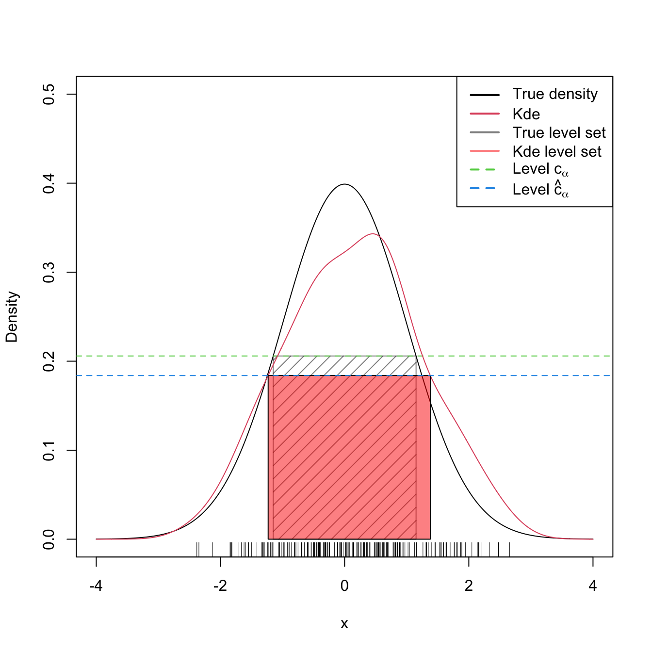

$Level set $\mathcal{L}(f;c_\alpha)$ and its estimation by $\mathcal{L}(\hat{f}(\cdot;h);\hat{c}_\alpha)$ for $\alpha=0.25$ and $f=\phi.$$

Figure 3.5: Level set $\mathcal{L}(f;c_\alpha)$ and its estimation by $\mathcal{L}(\hat{f}(\cdot;h);\hat{c}_\alpha)$ for $\alpha=0.25$ and $f=\phi.$

Observe that equation (3.19) points towards a simple way of approximating the multidimensional integral $\int_{\mathcal{L}(f;c)}f(\mathbf{x})\,\mathrm{d}\mathbf{x}$ throughout a sample $\mathbf{X}_1,\ldots,\mathbf{X}_n$ of $f$:

\[\begin{align} \int_{\mathcal{L}(f;c)}f(\mathbf{x})\,\mathrm{d}\mathbf{x}=\mathbb{P}[f(\mathbf{X})\geq c]\approx \frac{1}{n}\sum_{i=1}^n1_{\{f(\mathbf{X}_i)\geq c\}}.\tag{3.20} \end{align}\]

This Monte Carlo method has the important advantage of avoiding an expensive numerical integration. This is precisely the same advantage behind the approximation of $c_\alpha$ (essentially, such that $\int_{\mathcal{L}(f;c_\alpha)}f(\mathbf{x})\,\mathrm{d}\mathbf{x}=1-\alpha$ for $\alpha\in(0,1)$) by the $\alpha$-quantile of $f(\mathbf{X}_1),\ldots,f(\mathbf{X}_n).$

The application of (3.20) is illustrated below.

# N(0, 1) case
alpha <- 0.3
x_c <- qnorm(1 - alpha / 2)
c_alpha <- dnorm(x_c)
c_alpha
## [1] 0.2331588

# Approximates c_alpha
quantile(dnorm(samp), probs = alpha)
##       30% 
## 0.2043856

# True integral: 1 - alpha (by construction)
1 - 2 * pnorm(-x_c)
## [1] 0.7

# Monte Carlo integration, approximates 1 - alpha
mean(dnorm(samp) >= c_alpha)
## [1] 0.655

Exercise 3.13 Consider the kde for the faithful$eruptions dataset with a DPI bandwidth.

What is the estimation of the shortest set that contains the $50\%$ of the probability? And the $75\%$?
Compare the results obtained with the application of a boxplot. Which graphical analysis do you think is more informative?

Exercise 3.14 Repeat Exercise 3.13 with the data airquality$Wind.

Exercise 3.15 Section 2F in Tukey (1977) presents “the Rayleigh example” as an illustration of the weakness of box plots (referred to as “schematic plots” in Tukey’s terminology) for analyzing bimodal data. The weights of nitrogen obtained by Lord Rayleigh (table in page 49 in Tukey (1977)) are:

x <- c(2.30143, 2.29816, 2.30182, 2.29890, 2.31017,
       2.30986, 2.31010, 2.31001, 2.29889, 2.29940,
       2.29849, 2.29889, 2.31024, 2.31030, 2.31028)

Obtain the box plot of x. Do you see any interesting insights?
Compute $\hat h_{\mathrm{LSCV}}$ (beware of local minima) and draw a kde based on this bandwidth.
Estimate and plot the shortest sets containing $50\%$ and $75\%$ of the probability. What are your insights?

Exercise 3.16 Repeat Exercise 3.12 but now considering $\alpha=0.25,0.50$ and obtaining the corresponding $c_\alpha$ and $\hat{c}_\alpha.$ Compute $c_\alpha$ by Monte Carlo from (3.20) using $M=10,000$ replications.

Exercise 3.17 Adapt the function kde_level_set to:

Receive as main arguments a sample x and a bandwidth h, instead of a density object.
Use internally ks::kde instead of density.
Receive an $\alpha,$ instead of $c,$ and internally determine $\hat c_\alpha.$
Retain the functionality of kde_level_set and return also c_alpha_hat.

Call this new function kde_level_set2 and validate it with the examples seen so far.

Bivariate and trivariate level sets

The computation of bivariate and trivariate level sets is conceptually similar, but their parametrization and graphical display are more challenging. In $\mathbb{R}^2,$ the level sets are simply obtained from the contour levels of $\hat{f}(\cdot;\mathbf{H}),$ which is done easily with the ks package.

# Simulated sample from a mixture of normals
n <- 200
set.seed(123456)
mu <- c(2, 2)
Sigma1 <- diag(c(2, 2))
Sigma2 <- diag(c(1, 1))
samp <- rbind(mvtnorm::rmvnorm(n = n / 2, mean = mu, sigma = Sigma1),
              mvtnorm::rmvnorm(n = n / 2, mean = -mu, sigma = Sigma2))

# Level set of the true density at levels c
c <- c(0.01, 0.03)
x <- seq(-5, 5, by = 0.1)
xx <- as.matrix(expand.grid(x, x))
contour(x, x, 0.5 * matrix(mvtnorm::dmvnorm(xx, mean = mu, sigma = Sigma1) +
                             mvtnorm::dmvnorm(xx, mean = -mu, sigma = Sigma2),
                           nrow = length(x), ncol = length(x)),
        levels = c)

# Plot of the contour level
H <- ks::Hpi(x = samp)
kde <- ks::kde(x = samp, H = H)
plot(kde, display = "slice", abs.cont = c, add = TRUE, col = 4) # Argument
# "abs.cont" for specifying c rather than (1 - alpha) * 100 in "cont"
legend("topleft", lwd = 2, col = c(1, 4),
       legend = expression(L * "(" * f * ";" * c * ")",
                           L * "(" * hat(f) * "(" %.% ";" * H * "), " * c *")"))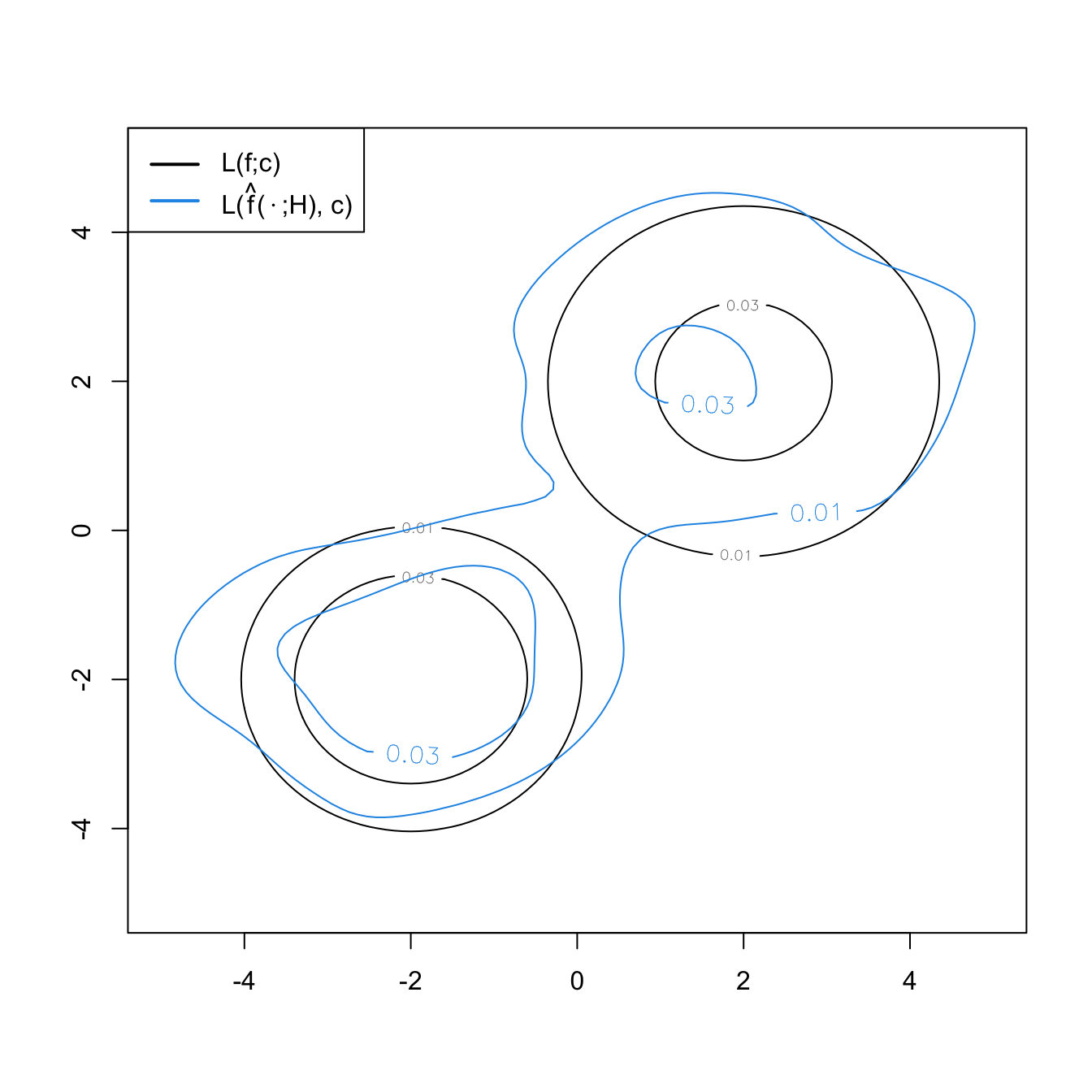


# Computation of the probability accumulated in the level sets by numerical
# integration
ks::contourSizes(kde, abs.cont = c)
## [1] 35.865815  7.321872

Exercise 3.18 Compute the level set containing the $50\%$ of the data of the following bivariate datasets: faithful, data(unicef, package = "ks"), and iris[, 1:2].

In $\mathbb{R}^3,$ the level sets are more challenging to visualize, as it is required to combine three-dimensional contours and the use of transparencies.

# Simulate a sample from a mixture of normals
n <- 5e2
set.seed(123456)
mu <- c(2, 2, 2)
Sigma1 <- rbind(c(1, 0.5, 0.2),
                c(0.5, 1, 0.5),
                c(0.2, 0.5, 1))
Sigma2 <- rbind(c(1, 0.25, -0.5),
                c(0.25, 1, 0.5),
                c(-0.5, 0.5, 1))
samp <- rbind(mvtnorm::rmvnorm(n = n / 2, mean = mu, sigma = Sigma1),
              mvtnorm::rmvnorm(n = n / 2, mean = -mu, sigma = Sigma2))

# Plot of the contour level, changing the color palette
H <- ks::Hns(x = samp)
kde <- ks::kde(x = samp, H = H)
plot(kde, cont = 100 * c(0.99, 0.95, 0.5), col.fun = viridis::viridis,
     drawpoints = TRUE, col.pt = 1, theta = 20, phi = 20)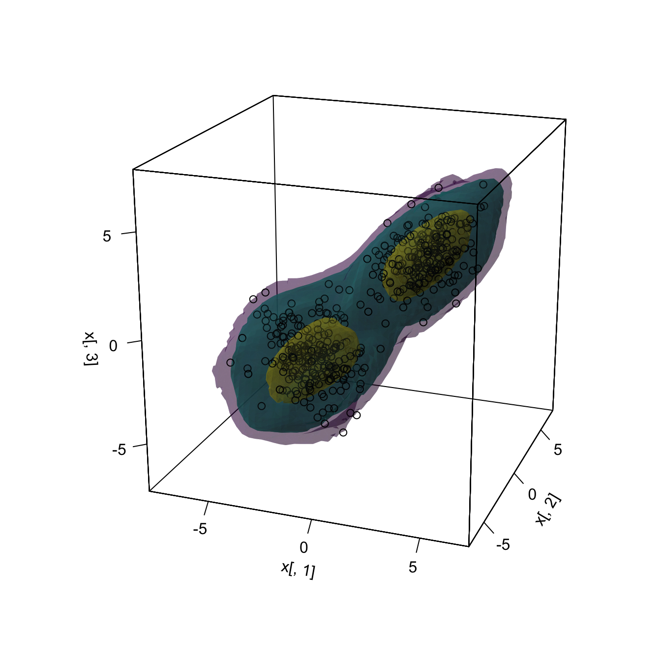

# Simulate a large sample from a single normal
n <- 5e4
set.seed(123456)
mu <- c(0, 0, 0)
Sigma <- rbind(c(1, 0.5, 0.2),
                c(0.5, 1, 0.5),
                c(0.2, 0.5, 1))
samp <- mvtnorm::rmvnorm(n = n, mean = mu, sigma = Sigma)

# Plot of the contour level
H <- ks::Hns(x = samp)
kde <- ks::kde(x = samp, H = H)
plot(kde, cont = 100 * c(0.75, 0.5, 0.25), xlim = c(-2.5, 2.5),
     ylim = c(-2.5, 2.5), zlim = c(-2.5, 2.5))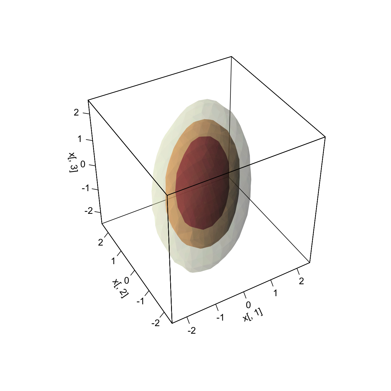

Support estimation and outlier detection

In addition to the highest density regions that accumulate $1-\alpha$ probability, for a relatively large $\alpha>0.5,$ it is also interesting to set $\alpha\approx0,$ as this gives an estimation of the effective support (excluding $\alpha$ probability) of $f.$ The estimated effective support of $\mathbf{X}$ gives valuable graphical insight into the structure of $\mathbf{X}$ and is helpful, for example, to determine the plausible region for data points coming from $f$ and then flag as outliers observations that fall outside the region, for arbitrary dimension.⁸³

The following code chunk shows how to compute estimates of the support in $\mathbb{R}^2$ via ks::ksupp.

# Compute kde of unicef dataset
data(unicef, package = "ks")
kde <- ks::kde(x = unicef)

# ks::ksupp evaluates whether the points in the grid spanned by ks::kde belong
# to the level set for alpha = 0.05 and then returns the points that belong to
# the level set (when convex.hull = FALSE)
supp <- as.matrix(ks::ksupp(fhat = kde, cont = 95, convex.hull = FALSE))
plot(supp) # Effective support except for a 5% of data

When dealing with sets defined by points on $\mathbb{R}^p,$ it is useful to consider the convex hull of the set of points, which is defined as the minor convex⁸⁴ set that contains all the points. The convex hull in $\mathbb{R}^2$ is computed with chull or by setting convex.hull = TRUE in ks::ksupp.

# The convex hull boundary of the level set can be computed with chull()
# It returns the indexes of the points passed that form the corners of the
# polygon of the convex hull
ch <- chull(supp)
plot(supp)
# One extra point for closing the polygon
lines(supp[c(ch, ch[1]), ], col = 2, lwd = 2)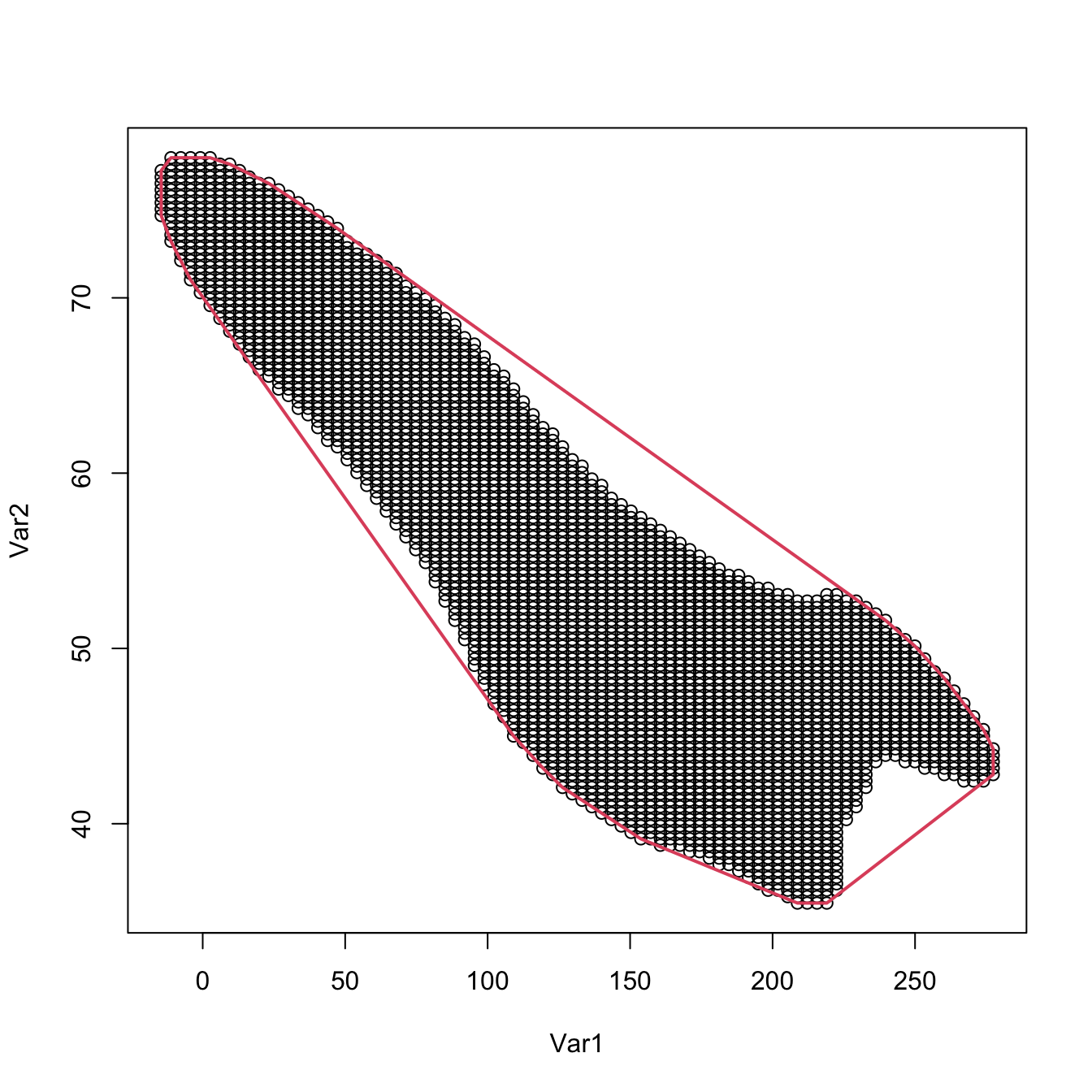


# Alternatively, use convex.hull = TRUE (default)
plot(supp)
plot(ks::ksupp(fhat = kde, cont = 95, convex.hull = TRUE),
     border = 3, lwd = 2)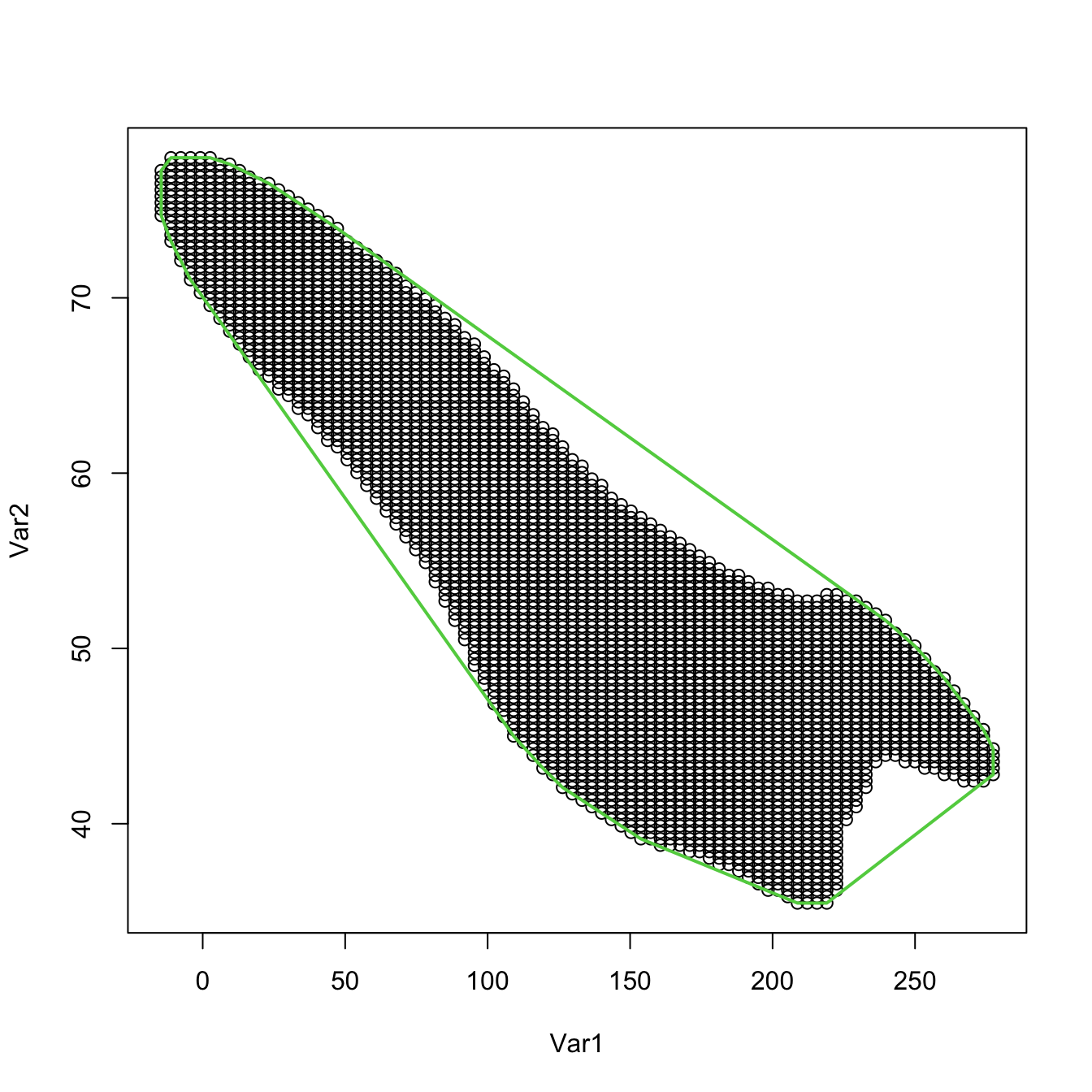

# The plotting method of ks::ksupp calls to polygon()

The convex hull may be seen as a conservative estimate of the effective support, since it may enlarge the level set estimation considerably. Another disadvantage is that it merges the individual components of unconnected supports. However, convex hulls pose interesting advantages: they can be computed in $\mathbb{R}^p$ via convex polyhedrons and then it is possible to check if a given point belongs to them. Thus, they give a handle to parametrize unknown-form level sets in $\mathbb{R}^p.$

These two functionalities are available in the geometry package⁸⁵ and have an interesting application: rather than evaluating if $\mathbf{x}\in\mathcal{L}(\hat{f}(\cdot;\mathbf{H});c),$ it is possible to just⁸⁶ check if $\mathbf{x}\in\mathrm{conv}(\{\mathbf{x}_1,\ldots,\mathbf{x}_N\}),$ where $\mathrm{conv}$ denotes the convex hull operator and $\{\mathbf{x}_1,\ldots,\mathbf{x}_N\}$ is a collection of points that roughly determines $\mathcal{L}(\hat{f}(\cdot;\mathbf{H});c).$ For example, the output of ks::ksupp in $\mathbb{R}^2$ or some points that belong to $\mathcal{L}(\hat{f}(\cdot;\mathbf{H});c)$ for $\mathbb{R}^p,$ $p\geq2.$

# Compute the convex hull of supp via geometry::convhulln()
C <- geometry::convhulln(p = supp)
# The output of geometry::convhulln() is different from chull()

# The geometry::inhulln() allows to check if points are inside the convex hull
geometry::inhulln(ch = C, p = rbind(c(50, 50), c(150, 50)))
## [1] FALSE  TRUE

# The convex hull works as well in R^p. An example in which the level set is
# evaluated by Monte Carlo and then the convex hull of the points in the level
# set is computed

# Sample
set.seed(2134)
samp <- mvtnorm::rmvnorm(n = 1e2, mean = rep(0, 3))

# Evaluation sample: random data in [-3, 3]^3
M <- 1e3
eval_set <- matrix(runif(n = 3 * M, -3, 3), M, 3)

# Kde of samp, evaluated at eval_set
H <- ks::Hns.diag(samp)
kde <- ks::kde(x = samp, H = H, eval.points = eval_set)

# Convex hull of points in the level set for a given c
c <- 0.01
C <- geometry::convhulln(p = eval_set[kde$estimate > c, ])

# We can test if a new point belongs to the level set by just checking if
# it belongs to the convex hull, which is much more efficient as it avoids
# re-evaluating the kde
new_points <- rbind(c(1, 1, 1), c(2, 2, 2))
geometry::inhulln(ch = C, p = new_points)
## [1]  TRUE FALSE
ks::kde(x = samp, H = H, eval.points = new_points)$estimate > c
## [1]  TRUE FALSE

# # Performance evaluation
# microbenchmark::microbenchmark(
#   geometry::inhulln(ch = C, p = new_points),
#   ks::kde(x = samp, H = H, eval.points = new_points)$estimate > c)

Detecting multivariate outliers in $\mathbb{R}^p$ is more challenging than in $\mathbb{R},$ and, unfortunately, the mere inspection of the marginals in the search for extreme values is not enough for successful outlier-hunting. A simple example in $\mathbb{R}^2$ is given in Figure 3.6.

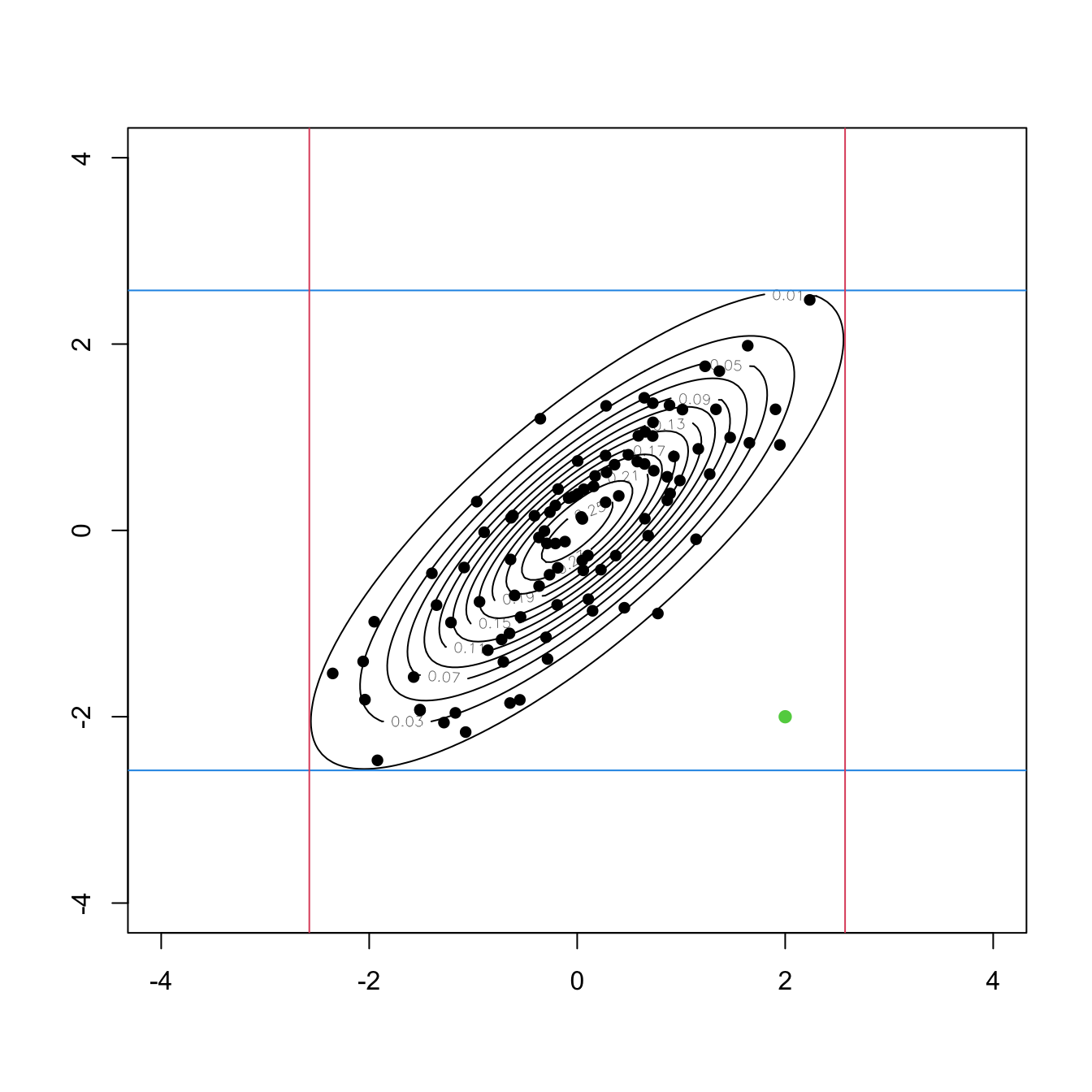
$An outlier (green point) in $\mathbb{R}^2$ that is not an outlier in any of the two marginals. The contour levels represent the joint density of a $\mathcal{N}_2(\mathbf{0},\boldsymbol{\Sigma}),$ where $\boldsymbol{\Sigma}$ is such that $\sigma^2_{11}=\sigma^2_{22}=1$ and $\sigma_{12}=0.8.$ The black points are sampled from that normal. The red and blue lines represent the $1-\alpha$ probability intervals $(-z_{\alpha/2},z_{\alpha/2})$ for $\alpha=0.01.$$

Figure 3.6: An outlier (green point) in $\mathbb{R}^2$ that is not an outlier in any of the two marginals. The contour levels represent the joint density of a $\mathcal{N}_2(\mathbf{0},\boldsymbol{\Sigma}),$ where $\boldsymbol{\Sigma}$ is such that $\sigma^2_{11}=\sigma^2_{22}=1$ and $\sigma_{12}=0.8.$ The black points are sampled from that normal. The red and blue lines represent the $1-\alpha$ probability intervals $(-z_{\alpha/2},z_{\alpha/2})$ for $\alpha=0.01.$

The next exercise shows an application of a level set estimation to outlier detection.

Exercise 3.19 Megaloblastic anemia is a kind of anemia that produces abnormally large red blood cells. Among others, indicators of megaloblastic anemia are low levels of: vitamin B12 (reference values: $178-1,100$ pg/ml), Folic Acid (FA; reference values: $>5.4$ ng), Mean Corpuscular Volume (MCV; reference values: $78-100$ fL), Hemoglobin (H; reference values: $13-17$ g/dL), and Iron (I; reference values: $60-160$ $\mu$g/dL). However, none can diagnose megaloblastic anemia by itself.

The dataset healthy-patients.txt contains realistically simulated data from $n_1=5,835$ blood analysis that include measurements for $\mathbf{X}=(\mathrm{B12}, \mathrm{FA}, \mathrm{MCV}, \mathrm{H}, \mathrm{I}),$ that is, a sample $\mathbf{X}_1,\ldots,\mathbf{X}_{n_1}.$ On the other hand, the dataset new-patients.txt contains observations of $\mathbf{X}$ for $n_2=117$ new patients, for which the presence of megaloblastic anemia is unknown. This sample is denoted by $\tilde{\mathbf{X}}_{1},\ldots,\tilde{\mathbf{X}}_{n_2}.$

Our aim is to identify outliers in this second dataset with respect to the first, in order to identify potential manifestations of megaloblastic anemia. To do so, we follow the following steps:

Obtain the normal scale bandwidth $\hat{\mathbf{H}}_\mathrm{NS}$ for the sample $\mathbf{X}_1,\ldots,\mathbf{X}_{n_1}.$
Obtain the level $\hat{c}_\alpha$ such that $0.995$ of the estimated probability of $\mathbf{X}$ is contained in $\mathcal{L}(\hat{f}(\cdot;\mathbf{H});\hat{c}_\alpha).$ Hint: recall how $\hat{c}_\alpha$ was defined.
Evaluate the kde $\hat{f}_i(\tilde{\mathbf{X}}_i;\hat{\mathbf{H}}_\mathrm{NS}),$ $i=1,\ldots,n_2,$ for the new sample $\tilde{\mathbf{X}}_1,\ldots,\tilde{\mathbf{X}}_{n_2},$ where $\hat{f}_i(\cdot;\hat{\mathbf{H}}_\mathrm{NS})$ stands for the kde of $\mathbf{X}_1,\ldots,\mathbf{X}_{n_1},\tilde{\mathbf{X}}_i.$⁸⁷
Check if $\hat{f}_i(\tilde{\mathbf{X}}_i;\hat{\mathbf{H}}_\mathrm{NS})<\hat{c}_\alpha,$ $i=1,\ldots,n,$ and flag $\tilde{\mathbf{X}}_{i}$ as an outlier if the condition holds.

Are there outliers? Do the observations flagged as outliers have the measurements inside the reference values?

Exercise 3.20 The wines.txt dataset contains chemical analyses of wines grown in Piedmont (Italy) coming from three different vintages: Nebbiolo, Barberas, and Grignolino. Perform a PCA after removing the vintage variable and standardizing the variables.

Considering the three first PCs, what is the smallest set that contains the $90\%$ of the probability? Represent the set graphically.
Is the point $\mathbf{x}_1=(0,-1.5,0)$ inside the level set? Could it be considered an outlier (remember the previous exercise)?
What about $\mathbf{x}_2=(2, -1.5, 2)$?
And what about $\mathbf{x}_3=(3, -3, 3)$?
Visualize the locations of $\mathbf{x}_1,$ $\mathbf{x}_2,$ and $\mathbf{x}_3$ to interpret the previous results

We conclude the section by highlighting a useful fact about the computation of areas under normal densities that is helpful to determine exactly the density levels for given probabilities. The density level $c_\alpha$ that contains $1-\alpha$ probability for $\mathbf{X}\sim\mathcal{N}_p(\boldsymbol{\mu},\boldsymbol{\Sigma})$ can be computed exactly by

\[\begin{align*} 1-\alpha=\mathbb{P}[\phi_{\boldsymbol\Sigma}(\mathbf{X}-\boldsymbol{\mu})\geq c]=\mathbb{P}\left[\chi^2_p\leq -2\log\left(|\boldsymbol{\Sigma}|^{1/2}(2\pi)^{p/2}c\right)\right], \end{align*}\]

since $(\mathbf{X}-\boldsymbol{\mu})'{\boldsymbol\Sigma}^{-1}(\mathbf{X}-\boldsymbol{\mu})\sim \chi_p^2.$ Therefore, for a given $\alpha\in(0,1)$

\[\begin{align} c_\alpha=|\boldsymbol{\Sigma}|^{-1/2}(2\pi)^{-p/2}e^{-\chi^2_{p;\alpha}/2},\tag{3.21} \end{align}\]

where $\chi^2_{p;\alpha}$ is the $\alpha$-upper quantile of a $\chi^2_p.$ The following code shows the computation of (3.21).

alpha <- 0.4
p <- 2
c_alpha <- exp(-0.5 * qchisq(p = 1 - alpha, df = p)) /
  (sqrt(det(Sigma)) * (2 * pi)^(p / 2))

3.5.2 Mean shift clustering

Perhaps one of the best-known clustering methods is $k$-means. Given a sample $\mathbf{X}_1,\ldots,\mathbf{X}_n$ in $\mathbb{R}^p,$ $k$-means is defined as the problem of finding the clusters $C_1,\ldots,C_k$ such that the within-cluster variation is as small as possible:

\[\begin{align*} \min_{C_1,\ldots,C_k}\left\{\sum_{j=1}^k \mathrm{W}(C_j)\right\} \end{align*}\]

where the within-cluster variation⁸⁸ of $C_j$ is defined as

\[\begin{align*} \mathrm{W}(C_j):=\frac{1}{|C_j|}\sum_{i,i'\in C_j} \|\mathbf{X}_i-\mathbf{X}_{i'}\|^2 \end{align*}\]

with $|C_j|:=\#\{i=1,\ldots,n:\mathbf{X}_i\in C_j\}$ denoting the number of observations in the $j$-th cluster.

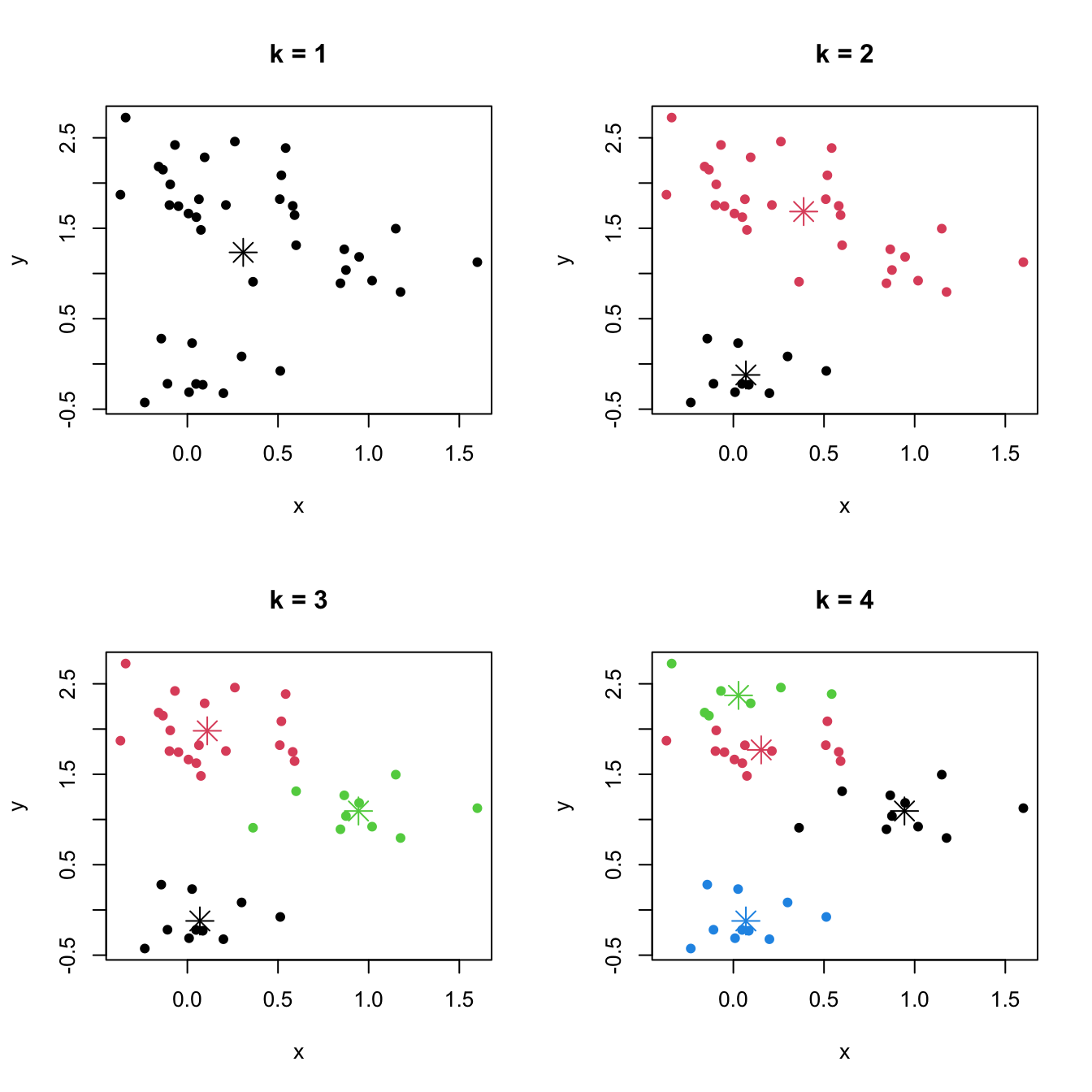
$$k$-means partitions for a two-dimensional dataset with $k=1,2,3,4.$ The center of each cluster is displayed with an asterisk.$

Figure 3.7: $k$-means partitions for a two-dimensional dataset with $k=1,2,3,4.$ The center of each cluster is displayed with an asterisk.

Behind the usefulness and simplicity of $k$-means hides an important drawback inherent to many clustering techniques: it is a method mostly defined on a sample basis⁸⁹ and for which a population analogue (in terms of the distribution of $\mathbf{X}$) is not clearly evident.⁹⁰ This has an important consequence: the somehow subjective concept of “cluster” depends on the observed sample, and thus there is no immediate objective definition in terms of the population.⁹¹ This implies that there is no clear population reference with which to compare the performance of a given sample clustering, that precise indications on the difficulty of performing clustering on a certain scenario are harder to make, and that there is no noticeable ground truth on what should be the right number of clusters for a given population.⁹²

$$k$-means partitions for $10,000$ observations sampled from the claw density for $k=5.$ Notice how despite the density’s having $5$ clear modes, the clusters are not associated with them (the blue on the right hand side captures the data on the right tail), even for the large sample size considered.$

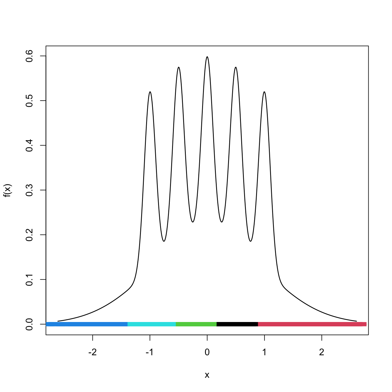
Figure 3.8: $k$-means partitions for $10,000$ observations sampled from the claw density for $k=5.$ Notice how despite the density’s having $5$ clear modes, the clusters are not associated with them (the blue on the right hand side captures the data on the right tail), even for the large sample size considered.

In the following, we study a principled population approach to clustering that tries to bypass these issues.

A population approach to clustering

The general goal of clustering, to find clusters of data with low within-cluster variation, can be regarded as the task of determining data-rich regions on the sample. From the density perspective, data-rich regions have a precise definition: modes and high-density regions. Therefore, modes are going to be crucial for defining population clusters in the sense introduced by Chacón (2015).

Given the random vector $\mathbf{X}$ in $\mathbb{R}^p$ with pdf $f,$ we denote the modes of $f$ by $\boldsymbol{\xi}_1,\ldots,\boldsymbol{\xi}_m.$ These are the local maxima of $f,$ i.e., $\mathrm{D}f(\boldsymbol{\xi}_j)=\mathbf{0},$ $j=1,\ldots,m.$ Intuitively, we can think of the population clusters as the regions of $\mathbb{R}^p$ that are “associated” with each of the modes of $f.$ This “association” can be visualized, for example, by a gravitational analogy: if $\boldsymbol{\xi}_1,\ldots,\boldsymbol{\xi}_m$ denote fixed equal-mass planets distributed on the space, then the population clusters can be thought of as the regions that determine the domains of attraction of each planet for an object $\mathbf{x}$ in the space that has zero initial speed. If $\mathbf{x}$ is attracted by $\boldsymbol{\xi}_1,$ then $\mathbf{x}$ belongs to the cluster defined by $\boldsymbol{\xi}_1.$ In our setting, the role of the gravity attraction is played by the gradient of the density $f,$ $\mathrm{D}f:\mathbb{R}^p\longrightarrow \mathbb{R}^p,$ which forms a vector field over $\mathbb{R}^p.$

The code below illustrates the previous analogy and serves to present the function numDeriv::grad.

# Planets
th <- 2 * pi / 3
r <- 2
xi_1 <- r * c(cos(th + 0.5), sin(th + 0.5))
xi_2 <- r * c(cos(2 * th + 0.5), sin(2 * th + 0.5))
xi_3 <- r * c(cos(3 * th + 0.5), sin(3 * th + 0.5))

# Gravity force
gravity <- function(x) {

  (mvtnorm::dmvnorm(x = x, mean = xi_1, sigma = diag(rep(0.5, 2))) +
     mvtnorm::dmvnorm(x = x, mean = xi_2, sigma = diag(rep(0.5, 2))) +
     mvtnorm::dmvnorm(x = x, mean = xi_3, sigma = diag(rep(0.5, 2)))) / 3

}

# Compute numerically the gradient of an arbitrary function
attraction <- function(x) numDeriv::grad(func = gravity, x = x)

# Evaluate the vector field
x <- seq(-4, 4, l = 20)
xy <- expand.grid(x = x, y = x)
dir <- apply(xy, 1, attraction)

# Scale arrows to unit length for better visualization
len <- sqrt(colSums(dir^2))
dir <- 0.25 * scale(dir, center = FALSE, scale = len)

# Colors of the arrows according to their original magnitude
brk <- quantile(len, probs = seq(0, 1, length.out = 21))
cuts <- cut(x = len, breaks = brk)
cols <- viridis::viridis(20)[cuts]

# Vector field plot
plot(0, 0, type = "n", xlim = c(-4, 4), ylim = c(-4, 4),
     xlab = "x", ylab = "y")
arrows(x0 = xy$x, y0 = xy$y,
       x1 = xy$x + dir[1, ], y1 = xy$y + dir[2, ],
       angle = 10, length = 0.1, col = cols, lwd = 2)
points(rbind(xi_1, xi_2, xi_3), pch = 19, cex = 1.5)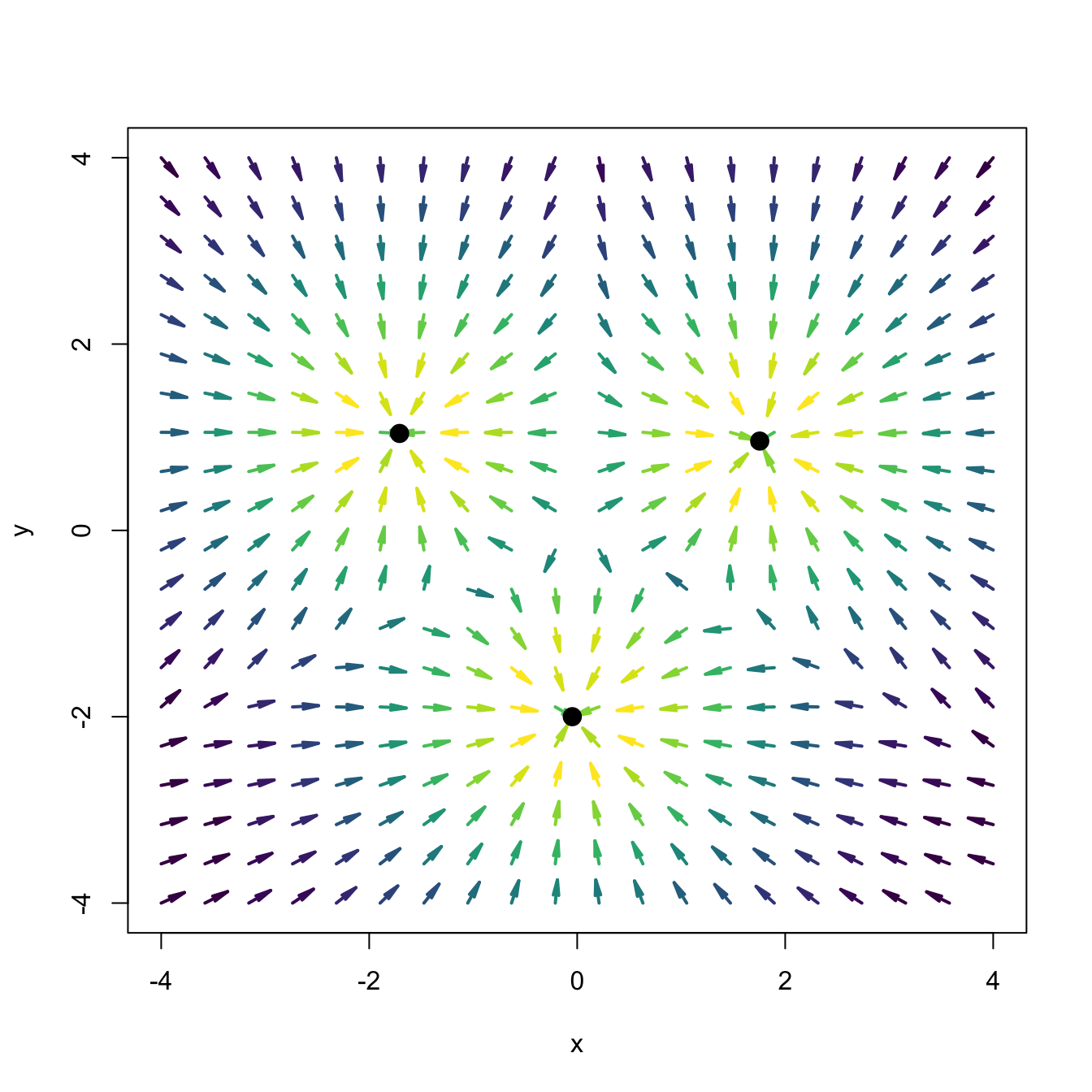

$Sketch of the gravity vector field associated with three equal-mass planets (black points). The vector field is computed as the gradient of a mixture of three bivariate normals centered at the black points and having covariance matrices $\frac{1}{2}\mathbf{I}_2.$ The direction of the arrows denotes the direction of the gravity field, and their color, the strength of the gravity force.$

Figure 3.9: Sketch of the gravity vector field associated with three equal-mass planets (black points). The vector field is computed as the gradient of a mixture of three bivariate normals centered at the black points and having covariance matrices $\frac{1}{2}\mathbf{I}_2.$ The direction of the arrows denotes the direction of the gravity field, and their color, the strength of the gravity force.

The previous idea can be mathematically formalized as follows. We seek to partition⁹³ $\mathbb{R}^p$ in a collection of disjoint subsets $W^s_+(\boldsymbol{\xi}_1),\ldots, W^s_+(\boldsymbol{\xi}_m)\,$⁹⁴ defined as

\[\begin{align*} W^s_+(\boldsymbol{\xi}):=\left\{\mathbf{x}\in\mathbb{R}^p:\lim_{t\to\infty}\boldsymbol{\phi}_{\mathbf{x}}(t)=\boldsymbol{\xi}\right\} \end{align*}\]

where $\boldsymbol{\phi}_{\mathbf{x}}:\mathbb{R}\longrightarrow\mathbb{R}^p$ is a curve in $\mathbb{R}^p$ parametrized by $t\in\mathbb{R}$ that satisfies the following Ordinal Differential Equation (ODE):

\[\begin{align} \frac{\mathrm{d}}{\mathrm{d}t}\boldsymbol{\phi}_{\mathbf{x}}(t)=\mathrm{D}f(\boldsymbol{\phi}_{\mathbf{x}}(t)),\quad \boldsymbol{\phi}_{\mathbf{x}}(0)=\mathbf{x}.\tag{3.22} \end{align}\]

This ODE admits a clear interpretation: the flow curve $\boldsymbol{\phi}_{\mathbf{x}}$ is the path that, originated at $\mathbf{x},$ describes $\mathbf{x}$ when reaching $\boldsymbol{\xi}_j$ through the direction of maximum ascent.⁹⁵ The ODE can be solved through different numerical schemes. For example, observing that $\frac{\mathrm{d}}{\mathrm{d}t}\boldsymbol{\phi}_{\mathbf{x}}(t)=\lim_{h\to0}\frac{\boldsymbol{\phi}_{\mathbf{x}}(t+h)-\boldsymbol{\phi}_{\mathbf{x}}(t)}{h},$ the Euler method considers the approximation

\[\begin{align} \boldsymbol{\phi}_{\mathbf{x}}(t+h)\approx\boldsymbol{\phi}_{\mathbf{x}}(t)+h\mathrm{D}f(\boldsymbol{\phi}_{\mathbf{x}}(t))\quad\text{if } h\approx 0,\tag{3.23} \end{align}\]

which motivates the iterative scheme⁹⁶

\[\begin{align} \begin{cases} \mathbf{x}_{t+1}=\mathbf{x}_t+h\mathrm{D}f(\mathbf{x}_t),\quad t=0,\ldots,N,\\ \mathbf{x}_{0}=\mathbf{x}, \end{cases} \tag{3.24} \end{align}\]

for a step $h>0$ and a number of maximum iterations $N.$

The following chunk of code illustrates the implementation of the Euler method (3.22) and gives insight into the paths $\boldsymbol{\phi}_{\mathbf{x}}.$ The code implements the exact gradient of a multivariate normal given in (3.9).

# Mixture parameters
mu_1 <- rep(1, 2)
mu_2 <- rep(-1.5, 2)
Sigma_1 <- matrix(c(1, -0.75, -0.75, 3), nrow = 2, ncol = 2)
Sigma_2 <- matrix(c(2, 0.75, 0.75, 3), nrow = 2, ncol = 2)
Sigma_1_inv <- solve(Sigma_1)
Sigma_2_inv <- solve(Sigma_2)
w <- 0.45

# Density
f <- function(x) {
  w * mvtnorm::dmvnorm(x = x, mean = mu_1, sigma = Sigma_1) +
    (1 - w) * mvtnorm::dmvnorm(x = x, mean = mu_2, sigma = Sigma_2)
}

# Gradient (caution: only works adequately for x a vector, it is not
# vectorized; observe that in the Sigma_inv %*% (x - mu) part the subtraction
# of mu and premultiplication by Sigma_inv are specific to a *single* point x)
Df <- function(x) {
  -(w * mvtnorm::dmvnorm(x = x, mean = mu_1, sigma = Sigma_1) *
      Sigma_1_inv %*% (x - mu_1) +
    (1 - w) * mvtnorm::dmvnorm(x = x, mean = mu_2, sigma = Sigma_2) *
      Sigma_2_inv %*% (x - mu_2))
}

# Plot density
ks::plotmixt(mus = rbind(mu_1, mu_2), Sigmas = rbind(Sigma_1, Sigma_2),
             props = c(w, 1 - w), display = "filled.contour2",
             gridsize = rep(251, 2), xlim = c(-5, 5), ylim = c(-5, 5),
             cont = seq(0, 90, by = 10), col.fun = viridis::viridis)

# Euler solution
x <- c(-2, 2)
# x <- c(-4, 0)
# x <- c(-4, 4)
N <- 1e3
h <- 0.5
phi <- matrix(nrow = N + 1, ncol = 2)
phi[1, ] <- x
for (t in 1:N) {

  phi[t + 1, ] <- phi[t, ] + h * Df(phi[t, ])# / f(phi[t, ])

}
lines(phi, type = "l")
points(rbind(x), pch = 19)
text(rbind(x), labels = "x", pos = 3)

# Mean of the components
points(rbind(mu_1, mu_2), pch = 16, col = 4)
text(rbind(mu_1, mu_2), labels = expression(mu[1], mu[2]), pos = 4, col = 4)

# The modes are different from the mean of the components! -- see the gradients
cbind(Df(mu_1), Df(mu_2))
##              [,1]         [,2]
## [1,] -0.005195479 1.528460e-04
## [2,] -0.002886377 7.132814e-05

# Modes
xi_1 <- optim(par = mu_1, fn = function(x) sum(Df(x)^2))$par
xi_2 <- optim(par = mu_2, fn = function(x) sum(Df(x)^2))$par
points(rbind(xi_1, xi_2), pch = 16, col = 2)
text(rbind(xi_1, xi_2), labels = expression(xi[1], xi[2]), col = 2, pos = 2)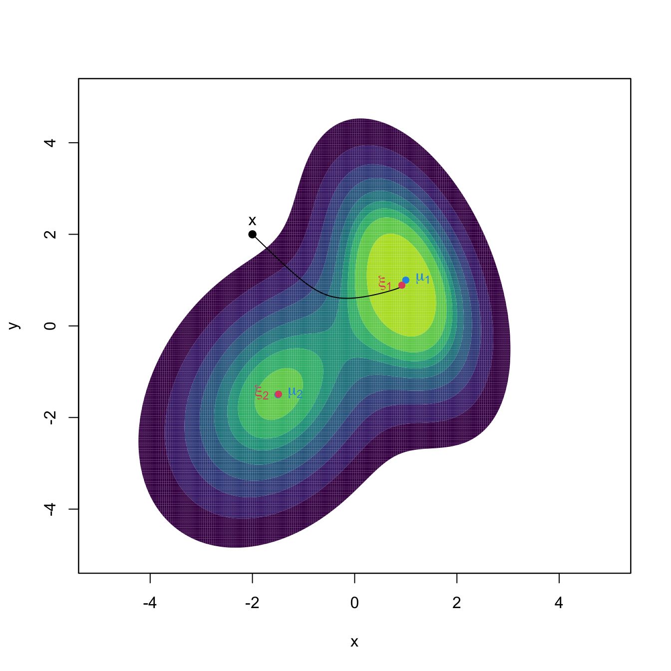

$The curve $\boldsymbol{\phi}_{\mathbf{x}}$ computed by the Euler method, in black. The population density is the mixture of bivariate normals $w\phi_{\boldsymbol{\Sigma}_1}(\cdot-\boldsymbol{\mu}_1)+(1-w)\phi_{\boldsymbol{\Sigma}_2}(\cdot-\boldsymbol{\mu}_2),$ where $\boldsymbol{\mu}_1=(1,1)',$ $\boldsymbol{\mu}_2=(-1.5,-1.5)',$ $\boldsymbol{\Sigma}_1=(1, -0.75; -0.75, 3),$ $\boldsymbol{\Sigma}_2=(2, 0.75; 0.75, 3),$ and $w=0.45.$ The component means $\boldsymbol{\mu}_1$ and $\boldsymbol{\mu}_2$ are shown in blue, whereas the two modes $\boldsymbol{\xi}_1$ and $\boldsymbol{\xi}_2$ of the density are represented in red. Note that the modes and the component means may be different.$

Figure 3.10: The curve $\boldsymbol{\phi}_{\mathbf{x}}$ computed by the Euler method, in black. The population density is the mixture of bivariate normals $w\phi_{\boldsymbol{\Sigma}_1}(\cdot-\boldsymbol{\mu}_1)+(1-w)\phi_{\boldsymbol{\Sigma}_2}(\cdot-\boldsymbol{\mu}_2),$ where $\boldsymbol{\mu}_1=(1,1)',$ $\boldsymbol{\mu}_2=(-1.5,-1.5)',$ $\boldsymbol{\Sigma}_1=(1, -0.75; -0.75, 3),$ $\boldsymbol{\Sigma}_2=(2, 0.75; 0.75, 3),$ and $w=0.45.$ The component means $\boldsymbol{\mu}_1$ and $\boldsymbol{\mu}_2$ are shown in blue, whereas the two modes $\boldsymbol{\xi}_1$ and $\boldsymbol{\xi}_2$ of the density are represented in red. Note that the modes and the component means may be different.

Exercise 3.21 Inspect the code generating Figure 3.10. Then:

Experiment with different values for the initial point $\mathbf{x}$ and inspect the resulting flow curves. What happens if $\mathbf{x}$ is in a low-density region?
Change the step $h$ to larger and smaller values. What happens? Has $h$ an influence on the convergence to a mode?
Does the “adequate” step $h$ depend on $\mathbf{x}$?

Clustering a sample: kernel mean shift clustering

From the previous example, it is clear how to assign a point $\mathbf{x}$ to a population cluster: compute its associated flow curve and assign the $j$-th cluster label if $\mathbf{x}\in W_+^s(\boldsymbol{\xi}_j).$ More importantly, once the population view of clustering is clear, performing clustering for a sample is conceptually trivial: just replace $f$ in (3.24) with its kde $\hat{f}(\cdot;\mathbf{H})$!⁹⁷ By doing so, it results that

\[\begin{align} \begin{cases} \mathbf{x}_{t+1}=\mathbf{x}_t+h\mathrm{D}\hat{f}(\mathbf{x}_t;\mathbf{H}),\quad t=0,\ldots,N,\\ \mathbf{x}_{0}=\mathbf{x}. \end{cases} \tag{3.25} \end{align}\]

A couple⁹⁸ more tweaks are required to turn (3.25) into a more practical relation. The first tweak boosts the travel through low-density regions and decreases the ascent at high-density regions (see Figure 3.11) by adapting the step size taken at $\mathbf{x}_{t+1}$ by the density at $\mathbf{x}_{t}.$ In version (3.24), this amounts to considering the normalized gradient⁹⁹

\[\begin{align*} \boldsymbol{\eta}(\mathbf{x}):=\frac{\mathrm{D}f(\mathbf{x})}{f(\mathbf{x})} \end{align*}\]

instead of the unnormalized gradient. Considering the normalized gradient can be seen as a replacement in (3.25) of the constant step $h$ by the variable step $h(\mathbf{x}):=a/f(\mathbf{x}),$ $a>0.$

$Comparison between unnormalized and normalized gradient vector fields. Observe how the unnormalized gradient almost vanishes at regions with low density and “overshoots” close to the modes. The normalized gradient gently adapts to the density region, boosting and slowing ascent as required. Both gradients have been standardized so that the norm of the maximum gradient is $2,$ therefore enabling their comparison.$ $Comparison between unnormalized and normalized gradient vector fields. Observe how the unnormalized gradient almost vanishes at regions with low density and “overshoots” close to the modes. The normalized gradient gently adapts to the density region, boosting and slowing ascent as required. Both gradients have been standardized so that the norm of the maximum gradient is $2,$ therefore enabling their comparison.$

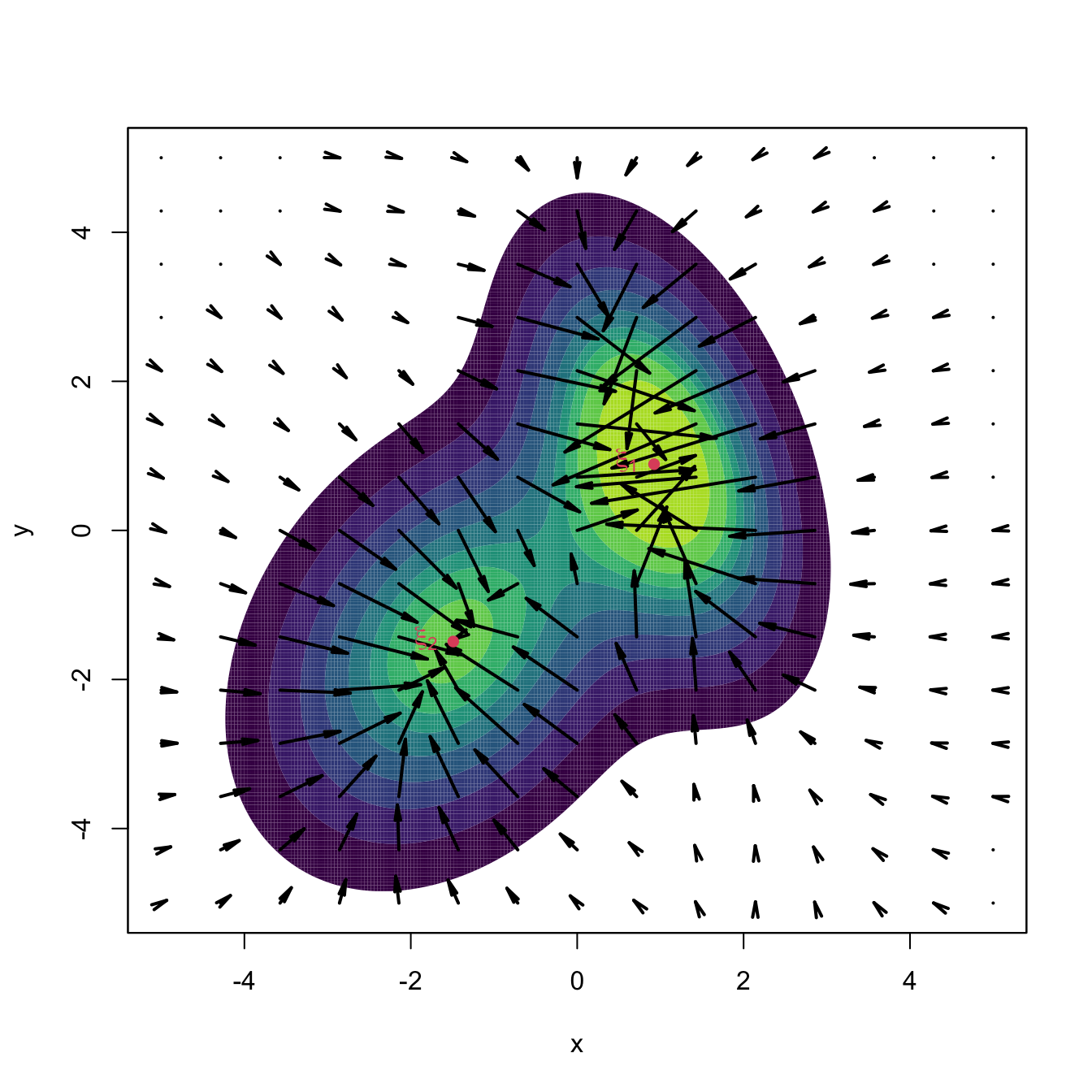
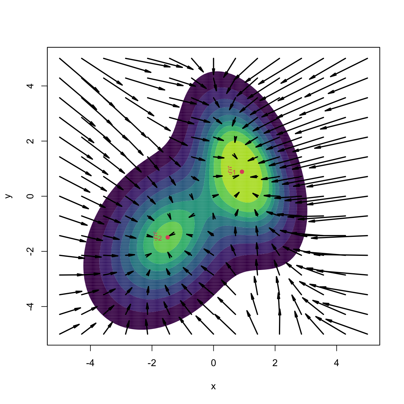
Figure 3.11: Comparison between unnormalized and normalized gradient vector fields. Observe how the unnormalized gradient almost vanishes at regions with low density and “overshoots” close to the modes. The normalized gradient gently adapts to the density region, boosting and slowing ascent as required. Both gradients have been standardized so that the norm of the maximum gradient is $2,$ therefore enabling their comparison.

The second tweak replaces $a$ in the variable step with a positive definite matrix $\mathbf{A}$ to premultiply $\boldsymbol{\eta}(\mathbf{x})$ and allow for more generality. This apparent innocuous change gives a convenient¹⁰⁰ choice for $\mathbf{A}$ and hence for the step in Euler’s method: $\mathbf{A}=\mathbf{H}.$

Joining the previous two tweaks, it results the recurrence relation of kernel mean shift clustering:

\[\begin{align} \mathbf{x}_{t+1}=\mathbf{x}_t+\mathbf{H}\hat{\boldsymbol{\eta}}(\mathbf{x}_t;\mathbf{H}),\quad \hat{\boldsymbol{\eta}}(\mathbf{x};\mathbf{H}):=\frac{\mathrm{D}\hat{f}(\mathbf{x};\mathbf{H})}{\hat{f}(\mathbf{x};\mathbf{H})}.\tag{3.26} \end{align}\]

The recipe for clustering a sample $\mathbf{X}_1,\ldots,\mathbf{X}_n$ is now simple:

Select a “suitable” bandwidth $\hat{\mathbf{H}}.$
For each element $\mathbf{X}_i,$ iterate the recurrence relation (3.26) “until convergence” to a given $\mathbf{y}_i,$ $i=1,\ldots,n.$
Find the set of “unique” end points $\{\boldsymbol{\xi}_1,\ldots,\boldsymbol{\xi}_m\}$ (the modes) among $\{\mathbf{y}_1,\ldots,\mathbf{y}_n\}.$
Label $\mathbf{X}_i$ as $j$ if it is associated with the $j$-th mode $\boldsymbol{\xi}_j.$

Some practical details are important when implementing the previous algorithm. First and more importantly, a “suitable” bandwidth $\hat{\mathbf{H}}$ has to be considered in order to carry out (3.26). Observe the crucial role of the bandwidth:

A large bandwidth $\hat{\mathbf{H}}$ will oversmooth the data and underestimate the number of modes. In the most extreme case, it will merge all the possible clusters into a single one positioned close to the sample mean $\bar{\mathbf{X}}.$
A small bandwidth $\hat{\mathbf{H}}$ will undersmooth the data, thus overestimating the number of modes. In the most extreme case, it will detect as many modes as data points.

The kind of bandwidth selectors recommended are the ones designed for gradient density estimation (see Sections 3.1 and 3.4), since (3.26) critically depends on estimating adequately the gradient (see discussion in Section 6.2.2 in Chacón and Duong (2018)). These bandwidth selectors yield larger bandwidths than the ones designed for density estimation (compare (3.18) with (3.17)).

In addition, both the iteration “until convergence” and the “uniqueness” of the end points¹⁰¹ have to be evaluated in practice with adequate numerical tolerances. The function ks::kms implements kernel mean shift clustering and automatically employs tested choices for numerical tolerances and convergence criteria.

# A simulated example for which the population clusters are known
# Extracted from ?ks::dmvnorm.mixt
mus <- rbind(c(-1, 0), c(1, 2 / sqrt(3)), c(1, -2 / sqrt(3)))
Sigmas <- 1/25 * rbind(ks::invvech(c(9, 63/10, 49/4)),
                       ks::invvech(c(9, 0, 49/4)),
                       ks::invvech(c(9, 0, 49/4)))
props <- c(3, 3, 1) / 7

# Sample the mixture
set.seed(123456)
x <- ks::rmvnorm.mixt(n = 1000, mus = mus, Sigmas = Sigmas, props = props)

# Kernel mean shift clustering. If H is not specified, then
# H = ks::Hpi(x, deriv.order = 1) is employed. Its computation may take some
# time, so it is advisable to compute it separately for later reuse
H <- ks::Hpi(x = x, deriv.order = 1)
kms <- ks::kms(x = x, H = H)

# Plot clusters
plot(kms, col = viridis::viridis(kms$nclust), pch = 19, xlab = "x", ylab = "y")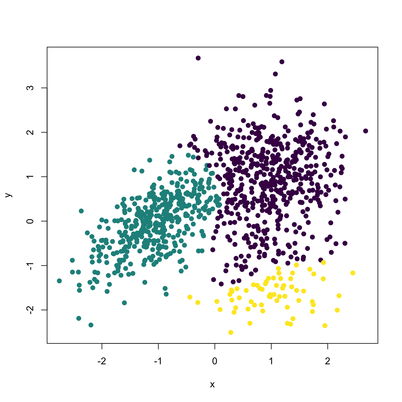


# Summary
summary(kms)
## Number of clusters = 3 
## Cluster label table = 521 416 63 
## Cluster modes =
##           V1          V2
## 1  1.0486466  0.96316436
## 2 -1.0049258  0.08419048
## 3  0.9888924 -1.43852908

# Objects in the kms object
kms$nclust # Number of clusters found
## [1] 3
kms$nclust.table # Sizes of clusters
## 
##   1   2   3 
## 521 416  63
kms$mode # Estimated modes
##            [,1]        [,2]
## [1,]  1.0486466  0.96316436
## [2,] -1.0049258  0.08419048
## [3,]  0.9888924 -1.43852908

# With keep.path = TRUE the ascending paths are returned
kms <- ks::kms(x = x, H = H, keep.path = TRUE)
cols <- viridis::viridis(kms$nclust, alpha = 0.5)[kms$label]
plot(x, col = cols, pch = 19, xlab = "x", ylab = "y")
for (i in 1:nrow(x)) lines(kms$path[[i]], col = cols[i])
points(kms$mode, pch = 8, cex = 2, lwd = 2)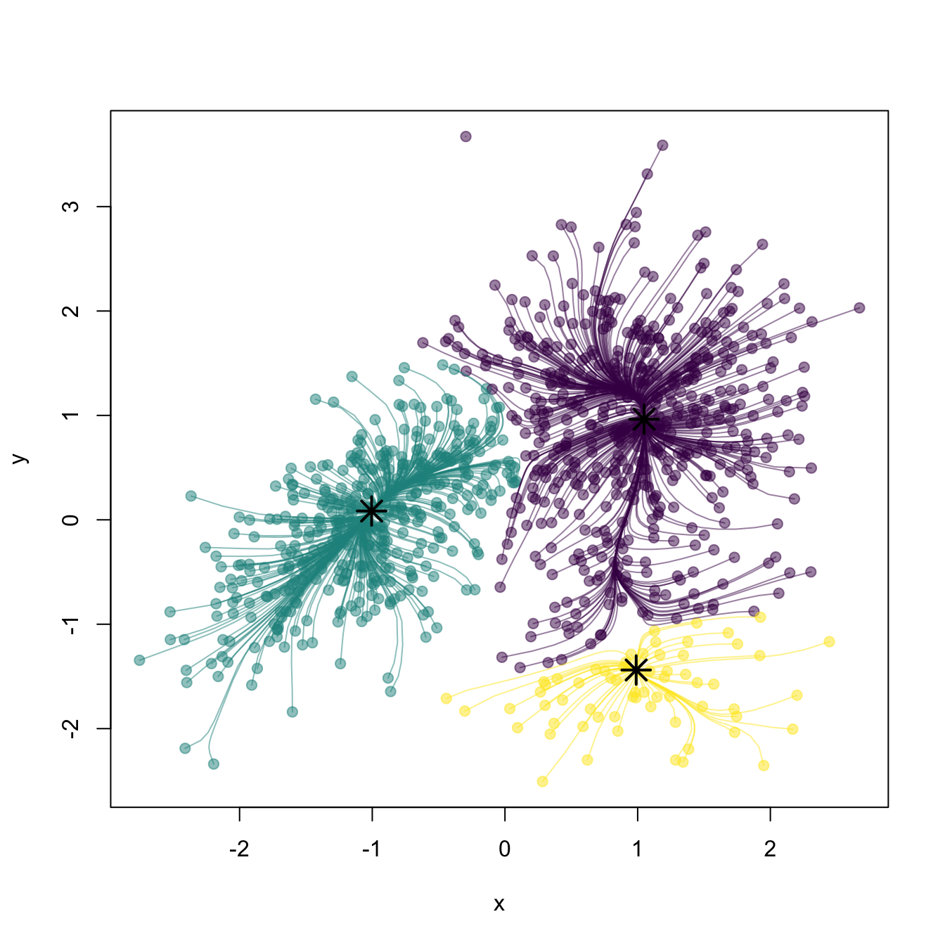

The partition of the whole space¹⁰² (not just the sample) can be done with ks::kms.part, whereas ks::mvnorm.mixt.part allows to partition the population if this is a mixture of normals.

# Partition of the whole sample space
kms_part <- ks::kms.part(x = x, H = H, xmin = c(-3, -3), xmax = c(3, 4),
                         gridsize = c(150, 150))
plot(kms_part, display = "filled.contour2", col = viridis::viridis(kms$nclust),
     xlab = "x", ylab = "y")
points(kms_part$mode, pch = 8, cex = 2, lwd = 2)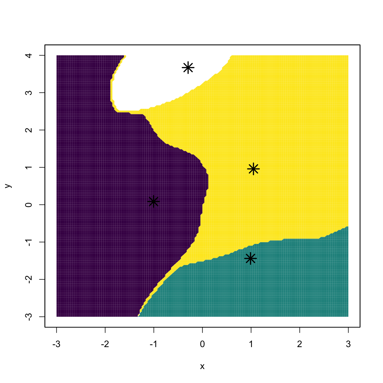


# Partition of the population
mixt_part <- ks::mvnorm.mixt.part(mus = mus, Sigmas = Sigmas, props = props,
                                  xmin = c(-3, -3), xmax = c(3, 4),
                                  gridsize = c(150, 150))
plot(mixt_part, display = "filled.contour2", col = viridis::viridis(kms$nclust),
     xlab = "x", ylab = "y")

# Obtain the modes of a mixture of normals automatically
modes <- ks::mvnorm.mixt.mode(mus = mus, Sigmas = Sigmas, props = props)
points(modes, pch = 8, cex = 2, lwd = 2)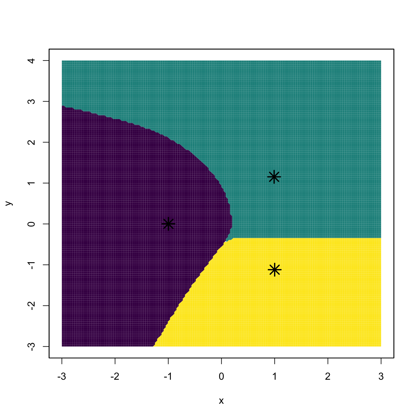

modes
##            [,1]         [,2]
## [1,] -0.9975330  0.002125069
## [2,]  0.9898321  1.153091638
## [3,]  0.9999969 -1.119886815
mus
##      [,1]      [,2]
## [1,]   -1  0.000000
## [2,]    1  1.154701
## [3,]    1 -1.154701

Finally, the ks::kms function is applied to the iris[, 1:3] dataset to illustrate a three-dimensional example.

# Obtain PI bandwidth
H <- ks::Hpi(x = iris[, 1:3], deriv.order = 1)

# Many (8) clusters: probably due to the repetitions in the data
kms_iris <- ks::kms(x = iris[, 1:3], H = H)
summary(kms_iris)
## Number of clusters = 8 
## Cluster label table = 47 3 25 11 55 3 3 3 
## Cluster modes =
##   Sepal.Length Sepal.Width Petal.Length
## 1     5.065099    3.442888     1.470614
## 2     5.783786    3.975575     1.255177
## 3     6.726385    3.026522     4.801402
## 4     5.576415    2.478507     3.861941
## 5     6.081276    2.884925     4.710959
## 6     6.168988    2.232741     4.310609
## 7     6.251387    3.375452     5.573491
## 8     7.208475    3.596510     6.118948

# Force to only find clusters that contain at least 10% of the data
# kms merges internally the small clusters with the closest ones
kms_iris <- ks::kms(x = iris[, 1:3], H = H, min.clust.size = 15)
summary(kms_iris)
## Number of clusters = 3 
## Cluster label table = 50 31 69 
## Cluster modes =
##   Sepal.Length Sepal.Width Petal.Length
## 1     5.065099    3.442888     1.470614
## 2     6.726385    3.026522     4.801402
## 3     5.576415    2.478507     3.861941

# Pairs plot -- good match of clustering with Species
plot(kms_iris, pch = as.numeric(iris$Species) + 1,
     col = viridis::viridis(kms_iris$nclust))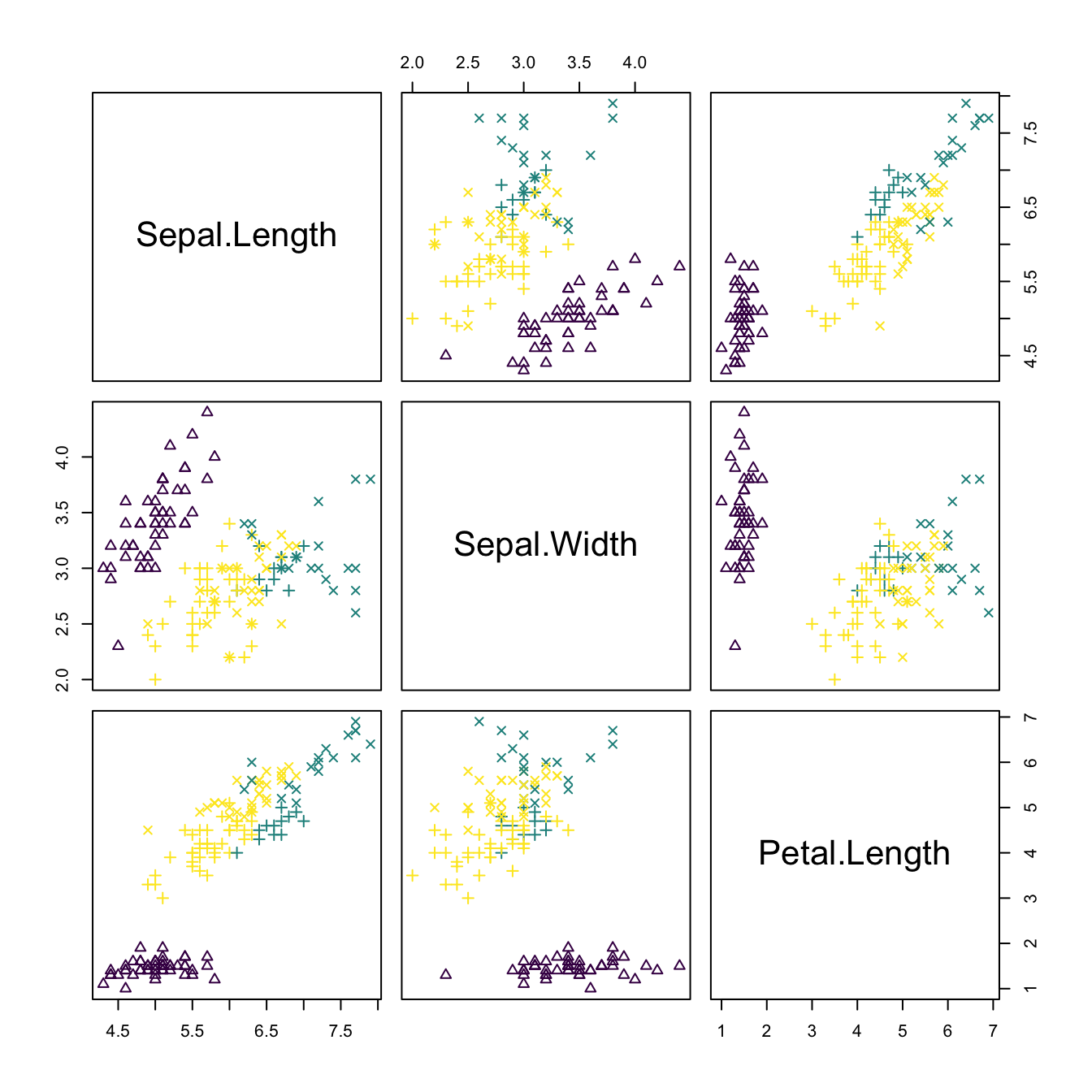

# See ascending paths
kms_iris <- ks::kms(x = iris[, 1:3], H = H, min.clust.size = 15,
                    keep.path = TRUE)
cols <- viridis::viridis(kms_iris$nclust)[kms_iris$label]
rgl::plot3d(kms_iris$x, col = cols)
for (i in 1:nrow(iris)) rgl::lines3d(kms_iris$path[[i]], col = cols[i])
rgl::points3d(kms_iris$mode, size = 5)
rgl::rglwidget()

Exercise 3.22 The dataset la-liga-2015-2016.xlsx contains team statistics for La Liga season 2015/2016.

How many clusters are detected for the variables Yellow.cards and Red.cards? And for Yellow.cards, Red.cards, and Fouls.made? Interpret the results.
Standardize the previous variables (divide them by their standard deviation) and recompute a. Are the results the same? Why? Does kmeans have a similar behavior?
Run a PCA on the dataset after removing Points and Matches and standardizing the variables. Then perform a clustering on the scores of as many PCs as to explain the $85\%$ of the variance. How many clusters are detected? What teams are associated with each of them? Are the clusters interpretable? Do you see something strange?
Run kmeans on the data used in c with $k=3,4,5$ and compare the results graphically.

Exercise 3.23 Load the wines.txt dataset and perform a PCA removing the vintage variable and after standardizing the variables.

How many clusters are detected using three PCs? What happens if min.clust.size is set such that the minimum cluster contains more than $5\%$ of the sample? Does it seem like a sensible choice to set such value of min.clust.size?
Using the same min.clust.size, consider six PCs. How many clusters are detected? Perform a pairs scatterplot and identify the PCs that are useful to identify clusters and the ones that seem to be adding noise.
Using the same min.clust.size, do the clustering with two PCs. How many clusters are now detected? Compare the clustering with two and three PCs. Why do you think there are fewer clusters in the latter? Hint: observe that the incremental information is on the scores of PC1 vs. PC3 and PC2 vs. PC3.
Compare the cluster made in part a with the variable vintages.
Run kmeans on the data used in part a with $k=3,4$ and compare the results graphically.

Exercise 3.24 Consider the MNIST dataset described in Exercise 2.25. Investigate the different ways of writing the digit “3” using kernel mean shift clustering. Follow the next steps:

Consider the $t$-SNE (van der Maaten and Hinton 2008) scores y_tsne of the class “3”. Use only the first $2,000$ $t$-SNE scores for the class “3” for the sake of computational expediency.
Compute the normal scale bandwidth matrix that is appropriate for performing kernel mean shift clustering with the first $2,000$ $t$-SNE scores.
Do kernel mean shift clustering on that subset using the previously obtained bandwidth and obtain the modes $\boldsymbol{\xi}_j,$ $j=1,\ldots,M,$ that cluster the $t$-SNE scores.
Determine the $M$ images that have the closest $t$-SNE scores, using the Euclidean distance, to the modes $\boldsymbol{\xi}_j.$
Show the closest images associated with the modes. Do they represent different forms of drawing the digit “3”?

3.5.3 Classification

We assume in this section that $\mathbf{X}$ has a categorical random variable $Y$ as a companion, the labels of $Y$ indicating one out of $m$ possible classes within the population $\mathbf{X},$ and that we have a sample $(\mathbf{X}_1,Y_1),\ldots,(\mathbf{X}_n,Y_n).$

Let’s denote $f_j$ to the conditional pdf of $\mathbf{X}|Y=j$ and $\pi_j$ to the value of the probability mass function of $Y$ at $j,$ i.e., $\mathbb{P}[Y=j]=\pi_j,$ for $j=1,\ldots, m.$ In this framework, the unconditional pdf $f$ of $\mathbf{X}$ is a mixture of the conditional pdfs. This is just a direct application of the law of the total probability:

\[\begin{align} f(\mathbf{x})=\sum_{j=1}^m f_j(\mathbf{x})\pi_j. \tag{3.27} \end{align}\]

The problem of assigning an observation $\mathbf{x}$ of $\mathbf{X}$ to each of the classes of $Y$ can be tackled by maximizing the conditional probability

\[\begin{align} \mathbb{P}[Y=j|\mathbf{X}=\mathbf{x}]&=\frac{f_j(\mathbf{x})\mathbb{P}[Y=j]}{f(\mathbf{x})}\nonumber\\ &=\frac{\pi_jf_j(\mathbf{x})}{\sum_{j=1}^m \pi_jf_j(\mathbf{x})},\tag{3.28} \end{align}\]

where a simple application of the Bayes’ rule involving pdfs and probabilities has been done in the first equality and (3.27) has been called in the second. The Bayes classifier exploits this idea of “assigning $\mathbf{x}$ to the most likely class $j$”:¹⁰³

\[\begin{align} \gamma_{\mathrm{Bayes}}(\mathbf{x}):=\arg\max_{j=1,\ldots,m} \pi_jf_j(\mathbf{x}).\tag{3.29} \end{align}\]

The Bayes classifier enjoys the minimum possible error rate among all possible classifiers. But, since it depends on the unknown $f_1,\ldots,f_m,\pi_1,\ldots,\pi_m,$ it can not be readily computed.

The solution now is evident: plug-in estimates for the unknown terms in (3.29) from the observed sample $(\mathbf{X}_1,Y_1),\ldots,(\mathbf{X}_n,Y_n).$ Estimating the class probabilities $\pi_j$ is simple: just consider their relative frequencies $\hat{\pi}_j:=\frac{n_j}{n},$ where $n_j:=\#\{i=1,\ldots,n:Y_i=j\}.$ Estimating $f_j$ can be done by a kde for the subsample $\{\mathbf{X}_i:Y_i=j,i=1,\ldots,n\},$ which we denote $\hat{f}_j(\cdot;\mathbf{H}_j).$ Plugging these estimates into (3.29) gives the kernel classifier

\[\begin{align} \hat{\gamma}(\mathbf{x};\mathbf{H}_1,\ldots,\mathbf{H}_m):=\arg\max_{j=1,\ldots,m} \hat{\pi}_j\hat{f}_j(\mathbf{x};\mathbf{H}_j).\tag{3.30} \end{align}\]

Application of (3.30) is often referred to as kernel discriminant analysis (kda).

The kernel classifier needs to be fed by the bandwidths $\mathbf{H}_1,\ldots,\mathbf{H}_m,$ each of them to be selected from each of the $m$ subsamples. However, these can be chosen by any of the procedures described in Section 3.4, as an adequate estimation of the conditional densities $f_j$ will yield sensible classification errors.¹⁰⁴ The main advantage of (3.30) with respect to classical LDA or QDA is the high flexibility induced by the natural nonlinearity of the classification frontier, which can capture any arbitrarily complicated form (yet retaining a conceptually simple formulation).

The ks::kda function implements kernel discriminant analysis. It essentially calls $m$ times to ks::kde in order to compute (3.30). In what follows the usage of ks::kda is illustrated, for $p=1,2,3,$ in the iris dataset.

# Univariate example
x <- iris$Sepal.Length
groups <- iris$Species

# By default, the ks::hpi bandwidths are computed
kda_1 <- ks::kda(x = x, x.group = groups)

# Manual specification of bandwidths via ks::hkda (we have univariate data)
hs <- ks::hkda(x = x, x.group = groups, bw = "plugin")
kda_1 <- ks::kda(x = x, x.group = groups, hs = hs)

# Estimated class probabilities
kda_1$prior.prob
## [1] 0.3333333 0.3333333 0.3333333

# Classification
head(kda_1$x.group.estimate)
## [1] setosa setosa setosa setosa setosa setosa
## Levels: setosa versicolor virginica

# (Training) classification error
ks::compare(x.group = kda_1$x.group, est.group = kda_1$x.group.estimate)
## $cross
##                   setosa (est.) versicolor (est.) virginica (est.) Total
## setosa (true)                45                 5                0    50
## versicolor (true)             6                28               16    50
## virginica (true)              1                10               39    50
## Total                        52                43               55   150
## 
## $error
## [1] 0.2533333

# Classification of new observations
ind_1 <- c(5, 55, 105)
newx <- x[ind_1]
predict(kda_1, x = newx)
## [1] setosa    virginica virginica
## Levels: setosa versicolor virginica
groups[ind_1] # Reality
## [1] setosa     versicolor virginica 
## Levels: setosa versicolor virginica

# Classification regions (points on the bottom)
plot(kda_1, xlab = "Sepal length", drawpoints = TRUE, col = rainbow(3))
legend("topright", legend = c("Setosa", "Versicolor", "Virginica"),
       lwd = 2, col = rainbow(3))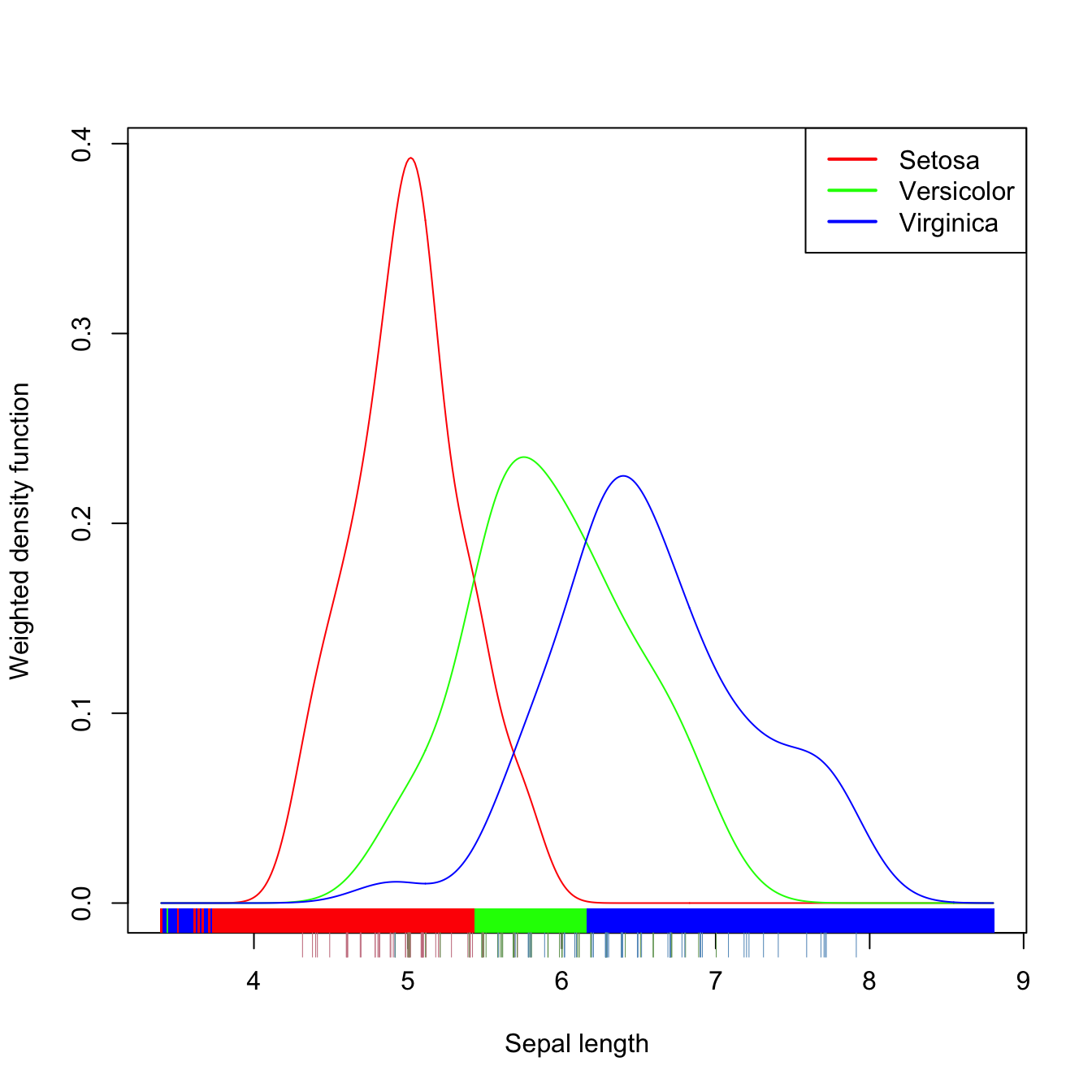

Figure 3.12: Discriminant regions classifying iris$Species from iris$Sepal.Length.

Exercise 3.25 Experiment with the code above by changing the variable Sepal.Length and the bandwidth selectors to see how the classification regions and errors change.

# Bivariate example
x <- iris[, 1:2]
groups <- iris$Species

# By default, the ks::Hpi bandwidths are computed
kda_2 <- ks::kda(x = x, x.group = groups)

# Manual specification of bandwidths via ks::Hkda
Hs <- ks::Hkda(x = x, x.group = groups, bw = "plugin")
kda_2 <- ks::kda(x = x, x.group = groups, Hs = Hs)

# Classification of new observations
ind_2 <- c(5, 55, 105)
newx <- x[ind_2, ]
predict(kda_2, x = newx)
## [1] setosa    virginica virginica
## Levels: setosa versicolor virginica
groups[ind_2] # Reality
## [1] setosa     versicolor virginica 
## Levels: setosa versicolor virginica

# Classification error
ks::compare(x.group = kda_2$x.group, est.group = kda_2$x.group.estimate)
## $cross
##                   setosa (est.) versicolor (est.) virginica (est.) Total
## setosa (true)                50                 0                0    50
## versicolor (true)             0                37               13    50
## virginica (true)              0                11               39    50
## Total                        50                48               52   150
## 
## $error
## [1] 0.16

# Plot of classification regions
plot(kda_2, col = rainbow(3), lwd = 2, col.pt = 1, cont = seq(5, 85, by = 20),
     col.part = rainbow(3, alpha = 0.25), drawpoints = TRUE)
# The artifacts on the corners (low-density regions) are caused by
# numerically-unstable divisions close to 0/0 

# The artifacts can be avoided by enlarging the effective support of the normal
# kernel that ks considers with supp (by default it is 3.7). Setting supp to
# a larger value (~10) will avoid the normal kernel to reach the value 0 
# exactly (but it may be required that the default gridsize has to be enlarged
# to display the surface adequately if supp is quite large). This is a useful
# practical tweak!
kda_2 <- ks::kda(x = x, x.group = groups, Hs = Hs, supp = 10)
plot(kda_2, col = rainbow(3), lwd = 2, col.pt = 1, cont = seq(5, 85, by = 20),
     col.part = rainbow(3, alpha = 0.25), drawpoints = TRUE)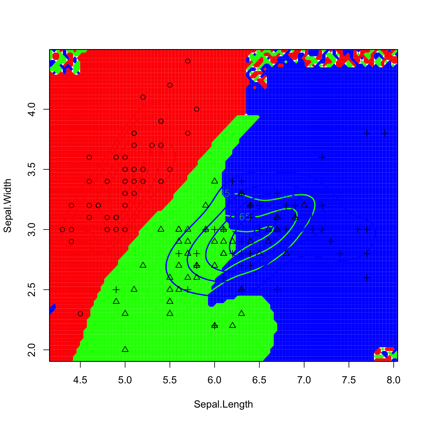

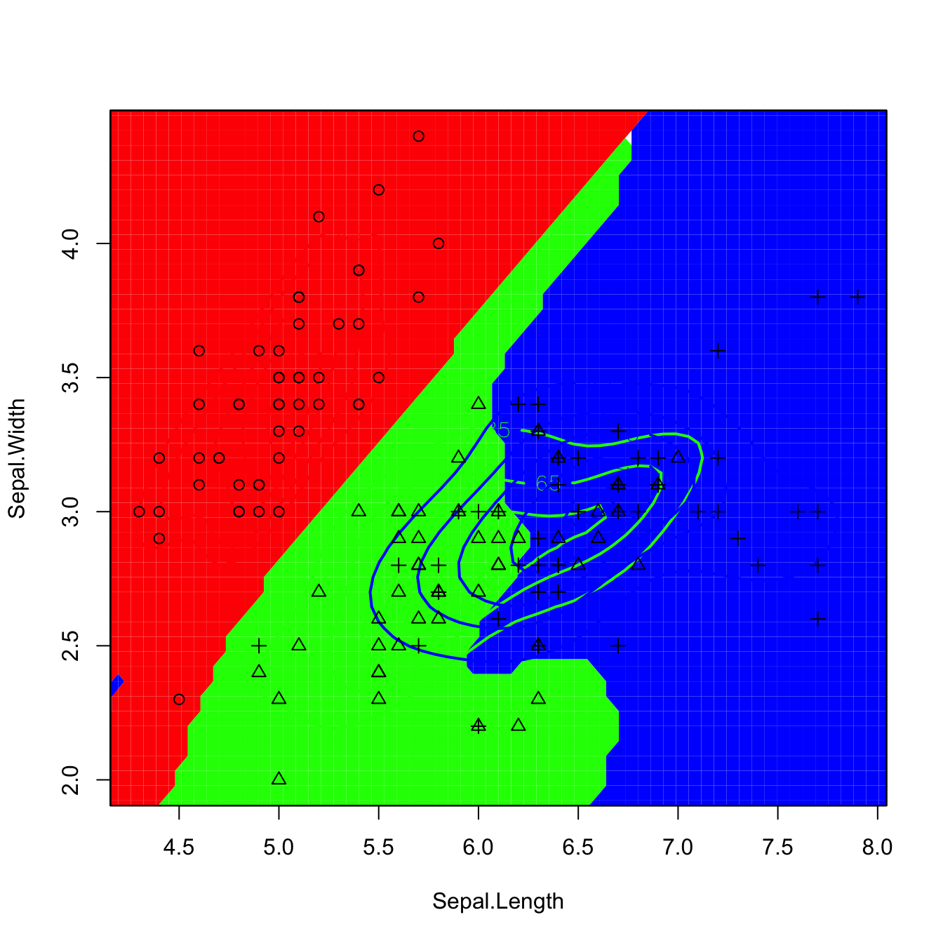
Discriminant regions classifying iris$Species from iris$Sepal.Length and iris$Sepal.Width. Observe that the second plot removes the artifacts of the former due to numerically-unstable divisions in low-density regions.

Figure 3.13: Discriminant regions classifying iris$Species from iris$Sepal.Length and iris$Sepal.Width. Observe that the second plot removes the artifacts of the former due to numerically-unstable divisions in low-density regions.

Exercise 3.26 Experiment with the previous code by changing the variables to see how the classification regions and errors change.

# Trivariate example
x <- iris[, 1:3]
groups <- iris$Species

# Normal scale bandwidths to avoid undersmoothing
Hs <- rbind(ks::Hns(x = x[groups == "setosa", ]),
            ks::Hns(x = x[groups == "versicolor", ]),
            ks::Hns(x = x[groups == "virginica", ]))
kda_3 <- ks::kda(x = x, x.group = groups, Hs = Hs)

# Classification of new observations
ind_3 <- c(5, 55, 105)
newx <- x[ind_3, ]
predict(kda_3, x = newx)
## [1] setosa     versicolor virginica 
## Levels: setosa versicolor virginica
groups[ind_3] # Reality
## [1] setosa     versicolor virginica 
## Levels: setosa versicolor virginica

# Classification regions
plot(kda_3, drawpoints = TRUE, col.pt = c(2, 3, 4), cont = seq(5, 85, by = 20),
     phi = 10, theta = 10)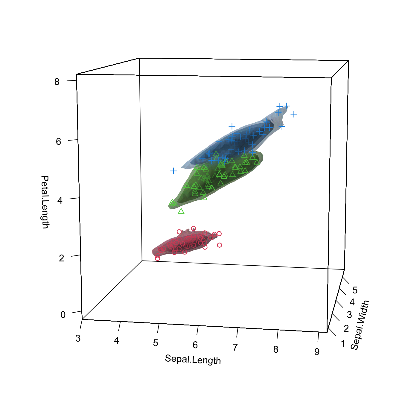

There was a bug in ks prior to 1.11.5, making ks::kda to work with equal-size classes only. Although the bug has been fixed, if you are experiencing problems applying ks::kda you can always apply several times ks::kde and compute (3.30) directly.

Exercise 3.27 Section 4.6.1 in James et al. (2013) considers the problem of classifying Direction from Lag1 and Lag2 (bivariate example) in data(Smarket, package = "ISLR") by logistic regression, LDA, and QDA.

Perform a kda and represent the classification regions. Do you think the classes can be separated effectively?
Split the dataset into train (Year < 2005) and test subsets. Obtain the global classification error rates on the test sample given by LDA and QDA (use MASS::lda and MASS::qda).
Obtain the global classification error rate on the test sample given by kda. Use directly the Bayes rule for performing classification.
Summarize the conclusions.

Use supp = 10 to avoid numerical artifacts.

Exercise 3.28 Load the wines.txt dataset and perform a PCA after removing the vintage variable and standardizing the variables. Then:

Perform a kda on the three classes of wines. First, use just the PC1 as covariate. Then, consider (PC1, PC2). Do you think the classes be separated effectively? With which information?
Compare the kda global classification error rates with those of LDA and QDA (use MASS::lda and MASS::qda).
Split the dataset into two thirds for training and one third for testing. Then compare the global classification error rates on the test sample for kda, LDA, and QDA. Again, first use just the PC1 as covariate, then consider (PC1, PC2).
Summarize the conclusions.

Exercise 3.29 Consider the MNIST dataset described in Exercise 2.25. Classify the digit images, via the $t$-SNE (van der Maaten and Hinton 2008) scores y_tsne, into the digit labels:

Split the dataset into the training sample, comprised of the first $50,000$ $t$-SNE scores and their associated labels, and the test sample (rest of the sample).
Using the training sample, compute the plug-in bandwidth matrices for all the classes.
Use these plug-in bandwidths to perform kernel discriminant analysis.
Plot the contours of the kernel density estimator of each class and overlay the $t$-SNE scores as points. Use coherent colors between contours and points, and add a legend.
Obtain the successful classification rate of the kernel discriminant analysis.

Exercise 3.30 Load the ovals.RData file.

Split the dataset into the training sample, comprised of the first $2,000$ observations, and the test sample (rest of the sample). Plot the dataset with colors for its classes. What can you say about the classification problem?
Using the training sample, compute the plug-in bandwidth matrices for all the classes.
Use these plug-in bandwidths to perform kernel discriminant analysis.
Plot the contours of the kernel density estimator of each class and the classes partitions. Use coherent colors between contours and points.
Predict the class for the test sample and compare with the true classes. Then report the successful classification rate.
Compare the successful classification rate with the one given by LDA. Is it better than kernel discriminant analysis?
Repeat f with QDA.

3.5.4 Density ridge estimation

PCA is a very well-known linear dimension-reduction technique that describes the main features of the data. From a population perspective, PCA is just an eigendecomposition of the covariance matrix $\boldsymbol{\Sigma}$ of a random vector $\mathbf{X}$:

\[\begin{align} \boldsymbol{\Sigma}=\mathbf{U}\boldsymbol{\Lambda}\mathbf{U}',\tag{3.31} \end{align}\]

where $\boldsymbol{\Lambda}=\mathrm{diag}(\lambda_1,\ldots,\lambda_p),$ $\lambda_1\geq \ldots\geq \lambda_p\geq0,$ and $\mathbf{U}=\left(\mathbf{u}_1,\ldots,\mathbf{u}_p\right)$ is an orthogonal matrix containing the principal components as column vectors. When $\mathbf{X}$ is centered,¹⁰⁵ the principal components give the directions of maximal projected variance of $\mathbf{X}.$ Therefore, PCA can always be computed for any random vector $\mathbf{X}$ with a proper covariance matrix $\boldsymbol{\Sigma}.$

It is however when $\mathbf{X}\sim\mathcal{N}_p(\mathbf{0},\boldsymbol{\Sigma})$ that PCA is especially meaningful. In that case, the eigendecomposition in (3.31) is related to the geometry of $\phi_{\boldsymbol{\Sigma}}$ by the search of the major and minor axes of the elliptical density contours. The relation between PCA and the normal distribution is not only geometrical, but also probabilistic: the principal components $\mathbf{U}$ can be reliably estimated by maximum likelihood, which amounts to performing the eigendecomposition (3.31) with $\boldsymbol{\Sigma}$ replaced with the sample covariance matrix¹⁰⁶ $\mathbf{S}.$ Therefore, for an arbitrary sample, performing PCA can be regarded as a three-step process: (i) fit a normal distribution with estimated variance $\mathbf{S};$ (ii) perform the eigendecomposition of $\mathbf{S};$ and (iii) attempt to reduce the dimensionality of the sample by discarding the principal components with smallest eigenvalues or projected variances.

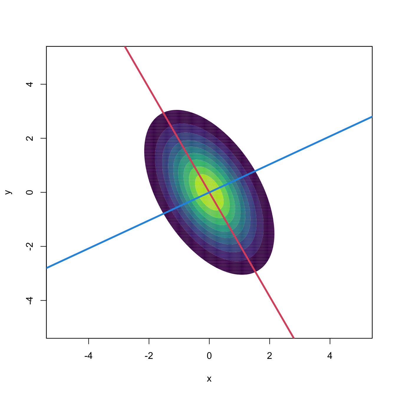
$Principal directions of $\mathcal{N}_2(\mathbf{0},\boldsymbol{\Sigma})$ with $\boldsymbol{\Sigma}=(1, -0.71; -0.71, 1).$ Red stands for PC1 and blue for PC2.$

Figure 3.14: Principal directions of $\mathcal{N}_2(\mathbf{0},\boldsymbol{\Sigma})$ with $\boldsymbol{\Sigma}=(1, -0.71; -0.71, 1).$ Red stands for PC1 and blue for PC2.

The takeaway of the previous discussion is that a popular dimension-reduction technique like PCA is closely related to the normal density; indeed, PCA can be regarded as a technique that rests on an assumption of normality for its accuracy. We next aim to remove this dependence of PCA on normality and to come up with a concept that extends the first principal direction shown in Figure 3.14 in a flexible way, giving a principal curve describing the main characteristics of any pdf $f.$

Density ridges

Approaching the example in Figure 3.14 from the three-dimensional views given in Figure 3.15 we can obtain a highly valuable insight for the PC1: it coincides with an “ascent path” to the “summit” (the mode) of the $\mathcal{N}_2(\mathbf{0},\boldsymbol{\Sigma})$’s pdf that is direct (no unnecessary detours), yet it is neither the steepest (the PC2 ascent is steeper) nor the one with fastest changes in the path’s slope.¹⁰⁷ That route follows the ridge¹⁰⁸ of the “mountain” given by $\phi_{\boldsymbol{\Sigma}}.$ Density ridges are a generalization of the concept of modes (indeed, any mode belongs to a density ridge) that may be relevant for summarizing the main features of a density.

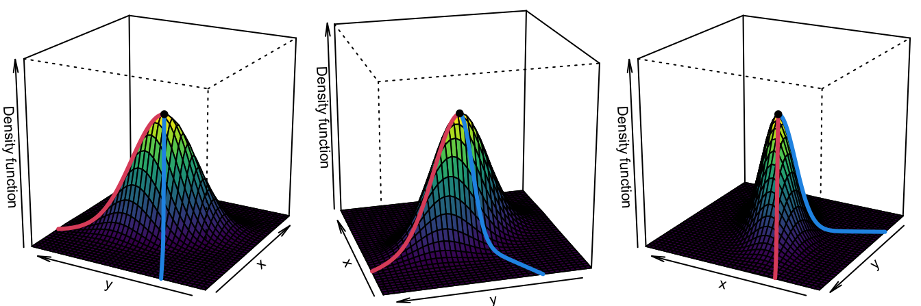
$PC1 “ascent path” (red) to the “summit” of a $\mathcal{N}_2(\mathbf{0},\boldsymbol{\Sigma})$’s pdf. The path precisely follows the ridge of $\phi_{\boldsymbol{\Sigma}}.$ Blue stands for the PC2 “ascent path”.$

Figure 3.15: PC1 “ascent path” (red) to the “summit” of a $\mathcal{N}_2(\mathbf{0},\boldsymbol{\Sigma})$’s pdf. The path precisely follows the ridge of $\phi_{\boldsymbol{\Sigma}}.$ Blue stands for the PC2 “ascent path”.

We define next what a density ridge is mathematically. We begin by considering the eigendecomposition of the Hessian matrix of a density function $f$ on $\mathbb{R}^p,$ $p\geq2,$ that is evaluated at $\mathbf{x}\in\mathbb{R}^p$:

\[\begin{align*} \mathrm{H} f(\mathbf{x}) = \mathbf{U}(\mathbf{x})\boldsymbol{\Lambda}(\mathbf{x})\mathbf{U}(\mathbf{x})', \end{align*}\]

where $\mathbf{U}(\mathbf{x})=\left(\mathbf{u}_1(\mathbf{x}), \ldots, \mathbf{u}_p(\mathbf{x})\right)$ and $\boldsymbol{\Lambda}(\mathbf{x})=\mathrm{diag}(\lambda_1(\mathbf{x}),\ldots,\lambda_p(\mathbf{x})),$ $\lambda_1(\mathbf{x})\geq \ldots\geq \lambda_p(\mathbf{x}).$ We denote $\mathbf{U}_{(p-1)}(\mathbf{x}):=\left(\mathbf{u}_2(\mathbf{x}),\ldots,\mathbf{u}_p(\mathbf{x}) \right)$ and define the projected gradient onto $\{\mathbf{u}_2(\mathbf{x}),\ldots,\mathbf{u}_p(\mathbf{x})\}$ as

\[\begin{align*} \mathrm{D}_{(p-1)}f(\mathbf{x}):=\mathbf{U}_{(p-1)}(\mathbf{x})\mathbf{U}_{(p-1)}(\mathbf{x})'\mathrm{D}f(\mathbf{x}), \end{align*}\]

which is a mapping $\mathrm{D}_{(p-1)}f:\mathbb{R}^p\longrightarrow\mathbb{R}^p.$ The density ridge of $f$ (or $1$-ridge of $f$), as defined by Genovese et al. (2014) (see also Section 6.3 in Chacón and Duong (2018)), consists of the set

\[\begin{align} \mathcal{R}_1(f):=\left\{\mathbf{x}\in\mathbb{R}^p:\|\mathrm{D}_{(p-1)}f(\mathbf{x})\|=0,\,\lambda_2(\mathbf{x})<0\right\}.\tag{3.32} \end{align}\]

This set may be comprised by the union of disjoint sets.

The intuition behind (3.32) as the precise definition for a density ridge is the following:

Ridges happen at regions that are locally maximal in certain directions, yet they may not necessarily be formed by local maxima (recall Figure 3.15). As a consequence, $\mathrm{H} f(\mathbf{x})$ is seminegative definite near a ridge, and so all the eigenvalues are non-positive: $\lambda_p(\mathbf{x})\leq\ldots\leq\lambda_1(\mathbf{x})\leq 0.$ Therefore, if $\lambda_1(\mathbf{x})\leq 0,$ the direction with largest negative curvature¹⁰⁹ is $\mathbf{u}_p,$ and $\mathbf{u}_1$ is the one with the least negative curvature.
$\mathrm{D}_{(p-1)}f(\mathbf{x})$ is the gradient projected onto the directions with largest negative curvatures (since we exclude $\mathbf{u}_1(\mathbf{x})$). When $\mathrm{D}_{(p-1)}f(\mathbf{x})=\mathbf{0},$ then either (1) $\mathrm{D}f(\mathbf{x})=\mathbf{0}$ or (2) $\mathrm{D}f(\mathbf{x})$ is orthogonal to $\mathbf{U}_{(p-1)}(\mathbf{x})\mathbf{U}_{(p-1)}(\mathbf{x})'.$
1. If $\mathrm{D}f(\mathbf{x})=\mathbf{0},$ then $\mathbf{x}$ is a relative extreme of $f,$ which could be a local maximum or a saddlepoint, since $\lambda_p(\mathbf{x})\leq\ldots\leq\lambda_2(\mathbf{x})<0,$ depending on the sign of $\lambda_1(\mathbf{x}).$ Modes and saddlepoints are actually part of ridges.
2. If $\mathrm{D}f(\mathbf{x})$ is orthogonal to $\mathbf{U}_{(p-1)}(\mathbf{x})\mathbf{U}_{(p-1)}(\mathbf{x})'$ then, in other words, it is parallel¹¹⁰ to $\mathbf{u}_1(\mathbf{x})$: $\mathrm{D}f(\mathbf{x})\propto \mathbf{u}_1(\mathbf{x}).$ Hence, the directions of maximum ascent and “maximum curvature” at $\mathbf{x}$ coincide.¹¹¹

The visualization of the construction of the vector field $\mathrm{D}_{(p-1)}f$ gives very valuable insights. In the following code, we rely on the functions grad_norm (computes $\mathrm{D}\phi_{\boldsymbol{\Sigma}}(\cdot-\boldsymbol{\mu})$) and Hess_norm (computes $\mathrm{H}\phi_{\boldsymbol{\Sigma}}(\cdot-\boldsymbol{\mu})$) defined on Section 3.2 to obtain proj_grad_norm (computes $\mathrm{D}_{(p-1)}\phi_{\boldsymbol{\Sigma}}(\cdot-\boldsymbol{\mu})$).

# Projected gradient into the Hessian s-th eigenvector subspace
proj_grad_norm <- function(x, mu, Sigma, s = 2) {

  # Gradient
  grad <- grad_norm(x = x, mu = mu, Sigma = Sigma)

  # Hessian
  Hess <- Hess_norm(x = x, mu = mu, Sigma = Sigma)

  # Eigenvectors Hessian
  eig_Hess <- t(apply(Hess, 3, function(A) {
    eigen(x = A, symmetric = TRUE)$vectors[, s]
  }))

  # Projected gradient
  proj_grad <- t(sapply(1:nrow(eig_Hess), function(i) {
    tcrossprod(eig_Hess[i, ]) %*% grad[i, ]
  }))

  # As an array
  return(proj_grad)

}

With the above functions, we can visualize the four vector fields $\mathbf{u}_1,\mathbf{u}_2,\mathrm{D}f,\mathrm{D}_{(p-1)}f:\mathbb{R}^p\longrightarrow\mathbb{R}^p,$ in $p=2,$ that are critical to construct density ridges.

# Compute vector fields
mu <- c(0, 0)
Sigma <- matrix(c(1, -0.71, -0.71, 3), nrow = 2, ncol = 2)
x <- seq(-3.5, 3.5, l = 12)
xx <- as.matrix(expand.grid(x, x))
H <- Hess_norm(x = xx, Sigma = Sigma, mu = mu)
eig_val_1 <- t(apply(H, 3, function(A) 
  eigen(x = A, symmetric = TRUE)$values[1]))
eig_val_2 <- t(apply(H, 3, function(A) 
  eigen(x = A, symmetric = TRUE)$values[2]))
eig_vec_1 <- t(apply(H, 3, function(A) 
  eigen(x = A, symmetric = TRUE)$vectors[, 1]))
eig_vec_2 <- t(apply(H, 3, function(A) 
  eigen(x = A, symmetric = TRUE)$vectors[, 2]))
grad <- grad_norm(x = xx, mu = mu, Sigma = Sigma)
grad_proj <- proj_grad_norm(x = xx, mu = mu, Sigma = Sigma)

# Standardize directions for nicer plots
r <- 0.5
eig_vec_1 <- r * eig_vec_1
eig_vec_2 <- r * eig_vec_2
grad <- r * grad / sqrt(rowSums(grad^2))
grad_proj <- r * grad_proj / sqrt(rowSums(grad_proj^2))

par(mfrow = c(2, 2))
ks::plotmixt(mus = mu, Sigmas = Sigma, props = 1, display = "filled.contour2",
             gridsize = rep(251, 2), xlim = c(-4, 4), ylim = c(-4, 4),
             cont = seq(0, 90, by = 10), col.fun = viridis::viridis,
             main = expression(bold(u)[1]))
arrows(x0 = xx[, 1], y0 = xx[, 2],
       x1 = xx[, 1] + eig_vec_1[, 1], y1 = xx[, 2] + eig_vec_1[, 2],
       length = 0.1, angle = 10, col = 1)
points(xx, pch = ifelse(eig_val_1 >= 0, "+", "-"),
       col = ifelse(eig_val_1 >= 0, 2, 4))

ks::plotmixt(mus = mu, Sigmas = Sigma, props = 1, display = "filled.contour2",
             gridsize = rep(251, 2), xlim = c(-4, 4), ylim = c(-4, 4),
             cont = seq(0, 90, by = 10), col.fun = viridis::viridis,
             main = expression(bold(u)[2]))
arrows(x0 = xx[, 1], y0 = xx[, 2],
       x1 = xx[, 1] + eig_vec_2[, 1], y1 = xx[, 2] + eig_vec_2[, 2],
       length = 0.1, angle = 10, col = 1)
points(xx, pch = ifelse(eig_val_2 >= 0, "+", "-"),
       col = ifelse(eig_val_2 >= 0, 2, 4))

ks::plotmixt(mus = mu, Sigmas = Sigma, props = 1, display = "filled.contour2",
             gridsize = rep(251, 2), xlim = c(-4, 4), ylim = c(-4, 4),
             cont = seq(0, 90, by = 10), col.fun = viridis::viridis,
             main = expression(plain(D) * f))
arrows(x0 = xx[, 1], y0 = xx[, 2],
       x1 = xx[, 1] + grad[, 1], y1 = xx[, 2] + grad[, 2],
       length = 0.1, angle = 10, col = 1)

ks::plotmixt(mus = mu, Sigmas = Sigma, props = 1, display = "filled.contour2",
             gridsize = rep(251, 2), xlim = c(-4, 4), ylim = c(-4, 4),
             cont = seq(0, 90, by = 10), col.fun = viridis::viridis,
             main = expression(plain(D)[(p - 1)] * f))
arrows(x0 = xx[, 1], y0 = xx[, 2],
       x1 = xx[, 1] + grad_proj[, 1], y1 = xx[, 2] + grad_proj[, 2],
       length = 0.1, angle = 10, col = 1)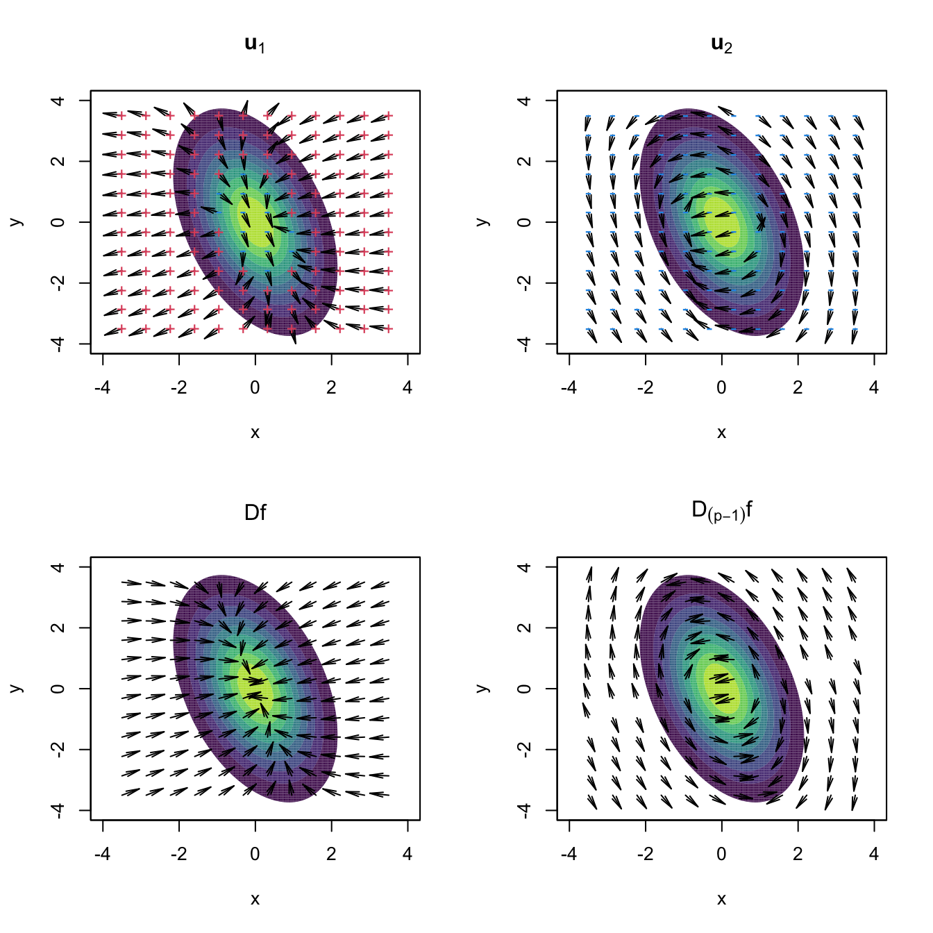

$Representation of the vector fields $\mathbf{u}_1,\mathbf{u}_2,\mathrm{D}f,\mathrm{D}_{(p-1)}f:\mathbb{R}^p\longrightarrow\mathbb{R}^p.$ Observe how the field $\mathrm{D}f$ pushes towards the mode but $\mathrm{D}_{(p-1)}f$ pushes towards the ridge, following the direction given by $\mathbf{u}_2.$ The field of $\mathbf{u}_1$ goes roughly right-to-left and parallel to the ridge, whereas the field of $\mathbf{u}_2$ goes roughly up-to-down and perpendicular to the ridge. The red plus (respectively, blue minus) indicate positive (negative) eigenvalue $\lambda_i(\mathbf{x})$ associated with $\mathbf{u}_i,$ $i=1,2$. The vector fields are normalized so that the norm of each vector is always the same.$

Figure 3.16: Representation of the vector fields $\mathbf{u}_1,\mathbf{u}_2,\mathrm{D}f,\mathrm{D}_{(p-1)}f:\mathbb{R}^p\longrightarrow\mathbb{R}^p.$ Observe how the field $\mathrm{D}f$ pushes towards the mode but $\mathrm{D}_{(p-1)}f$ pushes towards the ridge, following the direction given by $\mathbf{u}_2.$ The field of $\mathbf{u}_1$ goes roughly right-to-left and parallel to the ridge, whereas the field of $\mathbf{u}_2$ goes roughly up-to-down and perpendicular to the ridge. The red plus (respectively, blue minus) indicate positive (negative) eigenvalue $\lambda_i(\mathbf{x})$ associated with $\mathbf{u}_i,$ $i=1,2$. The vector fields are normalized so that the norm of each vector is always the same.

The construction of $\mathcal{R}_1(f)$ can be generalized to higher dimensions. The density $s$-ridge, $1\leq s\leq p-1,$ is defined as

\[\begin{align*} \mathcal{R}_s(f)=\{\mathbf{x}\in\mathbb{R}^p:\|\mathrm{D}_{(p-s)}f(\mathbf{x})\|=0,\,\lambda_{s+1}(\mathbf{x})<0\}, \end{align*}\]

where $\mathrm{D}_{(p-s)}f(\mathbf{x}):=\mathbf{U}_{(p-s)}(\mathbf{x})\mathbf{U}_{(p-s)}(\mathbf{x})'\mathrm{D}f(\mathbf{x})$ and $\mathbf{U}_{(p-s)}:=\left(\mathbf{u}_{s+1}(\mathbf{x}),\ldots,\mathbf{u}_p(\mathbf{x}) \right).$ The density $s$-ridge allows to summarize the main features of $f$ by surfaces of dimension $s,$ similarly to how the plane spanned by PC1 and PC2 describes most of the variability of a three-dimensional random variable $\mathbf{X}.$

We conclude by proving that, indeed, the density $1$-ridge of a $\mathcal{N}_p(\mathbf{0},\boldsymbol{\Sigma})$ is very related to the first principal direction PC1.

Proposition 3.1 Let $\boldsymbol{\Sigma}$ as in (3.31). Then $\left\{c\mathbf{u}_1:c\in\mathbb{R}\right\}\subset\mathcal{R}_1\left(\phi_{\boldsymbol{\Sigma}}\right).$

Proof. Consider (3.9) and (3.10) with $\boldsymbol{\mu}=\mathbf{0}$:

\[\begin{align*} \mathrm{D}\phi_{\boldsymbol{\Sigma}}(\mathbf{x})&=-\phi_{\boldsymbol{\Sigma}}(\mathbf{x})\boldsymbol{\Sigma}^{-1}\mathbf{x},\\ \mathrm{H}\phi_{\boldsymbol{\Sigma}}(\mathbf{x})&=\phi_{\boldsymbol{\Sigma}}(\mathbf{x})\left((\boldsymbol{\Sigma}^{-1}\mathbf{x})(\boldsymbol{\Sigma}^{-1}\mathbf{x})'-\boldsymbol{\Sigma}^{-1}\right). \end{align*}\]

Let’s take $\mathbf{x}=c\mathbf{u}_1,$ $c\in\mathbb{R},$ and show that $\mathrm{D}_{(p-1)}f(c\mathbf{u}_1)=\mathbf{0}$ and that the second eigenvalue of $\mathrm{H}\phi_{\boldsymbol{\Sigma}}(c \mathbf{u}_1)$ is negative.

Since $\boldsymbol{\Sigma}=\sum_{i=1}^p\lambda_i\mathbf{u}_i\mathbf{u}_i'$ and $\boldsymbol{\Sigma}^{-1}=\sum_{i=1}^p\lambda_i^{-1}\mathbf{u}_i\mathbf{u}_i',$ then

\[\begin{align} \mathrm{D}\phi_{\boldsymbol{\Sigma}}(c \mathbf{u}_1)=&-\phi_{\boldsymbol{\Sigma}}(c \mathbf{u}_1)c\lambda_1^{-1} \mathbf{u}_1,\tag{3.33}\\ \mathrm{H}\phi_{\boldsymbol{\Sigma}}(c \mathbf{u}_1)=&\,\phi_{\boldsymbol{\Sigma}}(c \mathbf{u}_1)\left(c^2\lambda_1^{-2} \mathbf{u}_1 \mathbf{u}_1'-\boldsymbol{\Sigma}^{-1}\right)\nonumber\\ =&\,\left(\phi_{\boldsymbol{\Sigma}}(c \mathbf{u}_1) \lambda_1^{-1}(c^2\lambda_1^{-1}-1)\right) \mathbf{u}_1 \mathbf{u}_1'\nonumber\\ &-\sum_{i=2}^p \left(\phi_{\boldsymbol{\Sigma}}(c \mathbf{u}_1)\lambda_i^{-1}\right)\mathbf{u}_i \mathbf{u}_i'.\tag{3.34} \end{align}\]

Therefore, $\mathrm{H}\phi_{\boldsymbol{\Sigma}}$ evaluated at $\mathbf{x}=c \mathbf{u}_1$ admits the eigendecomposition

\[\begin{align*} \mathrm{H}\phi_{\boldsymbol{\Sigma}}(c \mathbf{u}_1)=\mathbf{U}\boldsymbol{\Lambda}(c\mathbf{u}_1)\mathbf{U}' \end{align*}\]

with

\[\begin{align*} \boldsymbol{\Lambda}(c\mathbf{u}_1)=\phi_{\boldsymbol{\Sigma}}(c \mathbf{u}_1)\mathrm{diag}\left(\lambda_1^{-1}(c^2\lambda_1^{-1}-1),-\lambda_2^{-1},\ldots,-\lambda_p^{-1}\right). \end{align*}\]

And then, as a consequence, all but the first eigenvalue of $\mathrm{H}\phi_{\boldsymbol{\Sigma}}(c \mathbf{u}_1)$ are negative. Finally, joining (3.33) and (3.34),

\[\begin{align*} \mathrm{D}_{(p-1)}(c\mathbf{u}_1)&=\mathbf{U}_{(p-1)}\mathbf{U}_{(p-1)}'\mathrm{D} f(c\mathbf{u}_1)\\ &=\mathbf{U}_{(p-1)}\mathbf{U}_{(p-1)}'(-\phi_{\boldsymbol{\Sigma}}(c \mathbf{u}_1)c\lambda_1^{-1}) \mathbf{u}_1\\ &=\mathbf{0}, \end{align*}\]

which concludes the proof.

Density ridges from mean shift clustering

The definition (3.32) paves the way to determine the density ridges in an exactly analogous way to how modes were located in mean shift clustering: by flowing with the gradient. Figure 3.16 illustrates that now this flowing has to be done using the projected gradient flow $\mathrm{D}_{(p-1)}f$ until attaining $\mathbf{x}\in\mathbb{R}^p$ such that $\mathrm{D}_{(p-1)}f(\mathbf{x})=\mathbf{0}.$

More precisely, (3.32) can be parametrized as

\[\begin{align*} \mathcal{R}_1(f)=\left\{\mathbf{x}\in\mathbb{R}^p:\lim_{t\to\infty}\boldsymbol{\phi}_{\mathbf{x}_0}(t)=\mathbf{x},\,\mathbf{x}_0\in\mathbb{R}^p\right\}, \end{align*}\]

where $\boldsymbol{\phi}_{\mathbf{x}_0}:\mathbb{R}\longrightarrow\mathbb{R}^p$ is a curve in $\mathbb{R}^p$ that satisfies the ODE

\[\begin{align} \frac{\mathrm{d}}{\mathrm{d}t}\boldsymbol{\phi}_{\mathbf{x}_0}(t)=\mathrm{D}_{(p-1)}f(\boldsymbol{\phi}_{\mathbf{x}_0}(t)),\quad \boldsymbol{\phi}_{\mathbf{x}_0}(0)=\mathbf{x}_0,\tag{3.35} \end{align}\]

where $\mathbf{x}_0$ is any point in $\mathbb{R}^p.$ As done in (3.22), (3.35) can be numerically approached through the Euler method:

\[\begin{align} \mathbf{x}_{t+1}=\mathbf{x}_t+h\mathrm{D}_{(p-1)}f(\mathbf{x}_t),\quad t=0,\ldots,N,\tag{3.36} \end{align}\]

for a step $h>0$ and a number of maximum iterations $N.$ Considering the normalized gradient in (3.36)

\[\begin{align*} \boldsymbol{\eta}_{(p-1)}(\mathbf{x}):=\frac{\mathrm{D}_{(p-1)}f(\mathbf{x})}{f(\mathbf{x})}, \end{align*}\]

instead of the unnormalized gradient, helps adapting the step size $h$ conveniently.¹¹²

The following chunk of code illustrates the implementation of the Euler method (3.35), showing the paths $\boldsymbol{\phi}_{\mathbf{x}_0}$ for different $\mathbf{x}_0.$

mu <- c(0, 0)
Sigma <- matrix(c(1, -0.71, -0.71, 2), nrow = 2, ncol = 2)
ks::plotmixt(mus = mu, Sigmas = Sigma, props = 1, display = "filled.contour2",
             gridsize = rep(251, 2), xlim = c(-5, 5), ylim = c(-5, 5),
             cont = seq(0, 90, by = 10), col.fun = viridis::viridis)

# Euler solution
x0 <- as.matrix(expand.grid(seq(-3, 3, l = 12), seq(-3, 3, l = 12)))
x <- matrix(NA, nrow = nrow(x0), ncol = 2)
N <- 500
h <- 0.5
phi <- matrix(nrow = N + 1, ncol = 2)
eps <- 1e-4
for (i in 1:nrow(x0)) {

  # Move along the flow curve
  phi[1, ] <- x0[i, ]
  for (t in 1:N) {

    # Euler update
    phi[t + 1, ] <- phi[t, ] + 
      h * proj_grad_norm(phi[t, ], mu = mu, Sigma = Sigma) /
      mvtnorm::dmvnorm(x = phi[t, ], mean = mu, sigma = Sigma)

    # Stopping criterion (to save computing time!)
    abs_tol <- max(abs(phi[t + 1, ] - phi[t, ]))
    rel_tol <- abs_tol / max(abs(phi[t, ]))
    if (abs_tol < eps | rel_tol < eps) break

  }

  # Save final point
  x[i, ] <- phi[t + 1, , drop = FALSE]
  
  # Plot lines and x0
  lines(phi[1:(t + 1), ], type = "l")
  points(x0[i, , drop = FALSE], pch = 19)

}

# Plot final points
points(x, pch = 19, col = 2)

# Join the ridge points with lines in an automatic and sensible way:
# an Euclidean Minimum Spanning Tree (EMST) problem!
emst <- emstreeR::ComputeMST(x = x, verbose = FALSE)
segments(x0 = x[emst$from, 1], y0 = x[emst$from, 2],
         x1 = x[emst$to, 1], y1 = x[emst$to, 2], col = 2, lwd = 2)

$Curves $\boldsymbol{\phi}_{\mathbf{x}_0}$ computed by the Euler method, in black. The population density is $\phi_{\boldsymbol{\Sigma}}(\cdot-\boldsymbol{\mu}),$ where $\boldsymbol{\mu}=(0,0)'$ and $\boldsymbol{\Sigma}=(1, -0.71; -0.71, 2).$ The initial points $\mathbf{x}_0$ are shown in black, whereas ridge points $\mathbf{x}$ are represented in red and are joined by the Euclidean minimum spanning tree (red line).$

Figure 3.17: Curves $\boldsymbol{\phi}_{\mathbf{x}_0}$ computed by the Euler method, in black. The population density is $\phi_{\boldsymbol{\Sigma}}(\cdot-\boldsymbol{\mu}),$ where $\boldsymbol{\mu}=(0,0)'$ and $\boldsymbol{\Sigma}=(1, -0.71; -0.71, 2).$ The initial points $\mathbf{x}_0$ are shown in black, whereas ridge points $\mathbf{x}$ are represented in red and are joined by the Euclidean minimum spanning tree (red line).

Of course, we can compute the ridges of arbitrary density functions using (3.36). Figure 3.18 shows the density ridges of several heavily non-normal densities.¹¹³ The figure also illustrates some practical problems that may appear when computing density ridges, even at the population level.

# "Oval" density
f_oval <- function(x, mu = 2, sigma = 0.35, 
                   Sigma = rbind(c(1, -0.71), c(-0.71, 2))) {

  # x always as a matrix
  x <- rbind(x)
  
  # Rotate x with distortion
  Sigma_inv_sqrt <- solve(chol(Sigma))
  x <- x %*% Sigma_inv_sqrt

  # Polar coordinates
  r <- sqrt(rowSums(x^2))

  # Density as conditional * marginal
  f_theta <- 1 / (2 * pi)
  f_r_theta <- dnorm(x = r, mean = mu, sd = sigma)
  jacobian <-  det(Sigma_inv_sqrt) / r
  f <- f_r_theta * f_theta * jacobian
  return(f)

}

# "Croissant" density
f_crois <- function(x, mu = 2, sigma = 0.5, mu_theta = pi / 2, kappa = 1) {

  # x always as a matrix
  x <- rbind(x)

  # Polar coordinates
  theta <- atan2(x[, 2], x[, 1])
  r <- sqrt(rowSums(x^2))

  # Density as conditional * marginal
  f_theta <- exp(kappa * cos(theta - mu_theta)) / 
    (2 * pi * besselI(kappa, nu = 0))
  f_r_theta <- dnorm(x = r, mean = mu, sd = sigma)
  jacobian <- 1 / r
  f <- f_r_theta * f_theta * jacobian
  return(f)

}

# "Sin" density
f_sin <- function(x, a = 0.5, b = 1.75, sigma_x = 2, sigma_y = 0.5) {

  # x always as a matrix
  x <- rbind(x)

  # Density as conditional * marginal
  f_y <- dnorm(x = x[, 1], mean = 0, sd = sigma_x)
  f_x_y <- dnorm(x = x[, 2], mean = a * (1 + x[, 1]) * sin(b * x[, 1]),
                 sd = sigma_y)
  f <- f_x_y * f_y
  return(f)

}

$Highly non-normal densities and the construction of their density ridges. In blue, the points $\mathbf{x}_0$ that lie on low-density regions and are skipped from the Euler algorithm (longer running times and not useful output). In red, the final points $\mathbf{x}$ that lie on ridges on high-density regions (thus excluding ill-defined ridges). The red line is the Euclidean minimum spanning tree of the final points.$ $Highly non-normal densities and the construction of their density ridges. In blue, the points $\mathbf{x}_0$ that lie on low-density regions and are skipped from the Euler algorithm (longer running times and not useful output). In red, the final points $\mathbf{x}$ that lie on ridges on high-density regions (thus excluding ill-defined ridges). The red line is the Euclidean minimum spanning tree of the final points.$ $Highly non-normal densities and the construction of their density ridges. In blue, the points $\mathbf{x}_0$ that lie on low-density regions and are skipped from the Euler algorithm (longer running times and not useful output). In red, the final points $\mathbf{x}$ that lie on ridges on high-density regions (thus excluding ill-defined ridges). The red line is the Euclidean minimum spanning tree of the final points.$

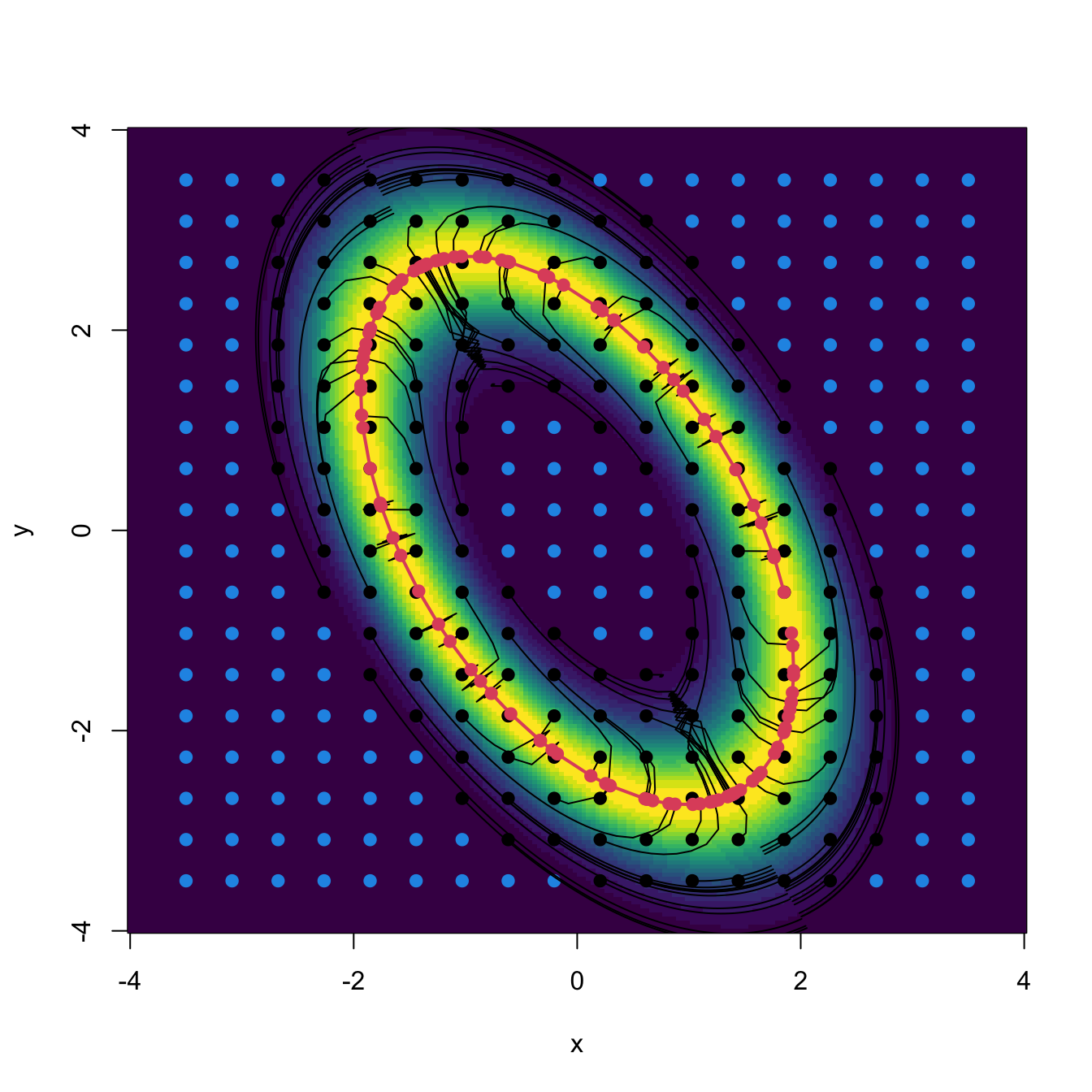
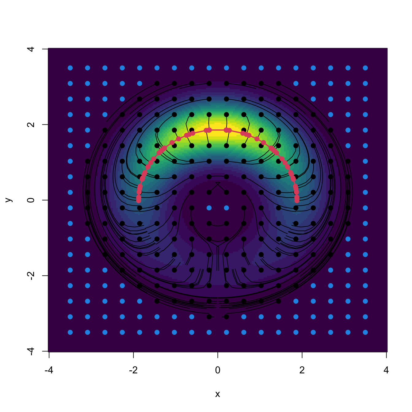
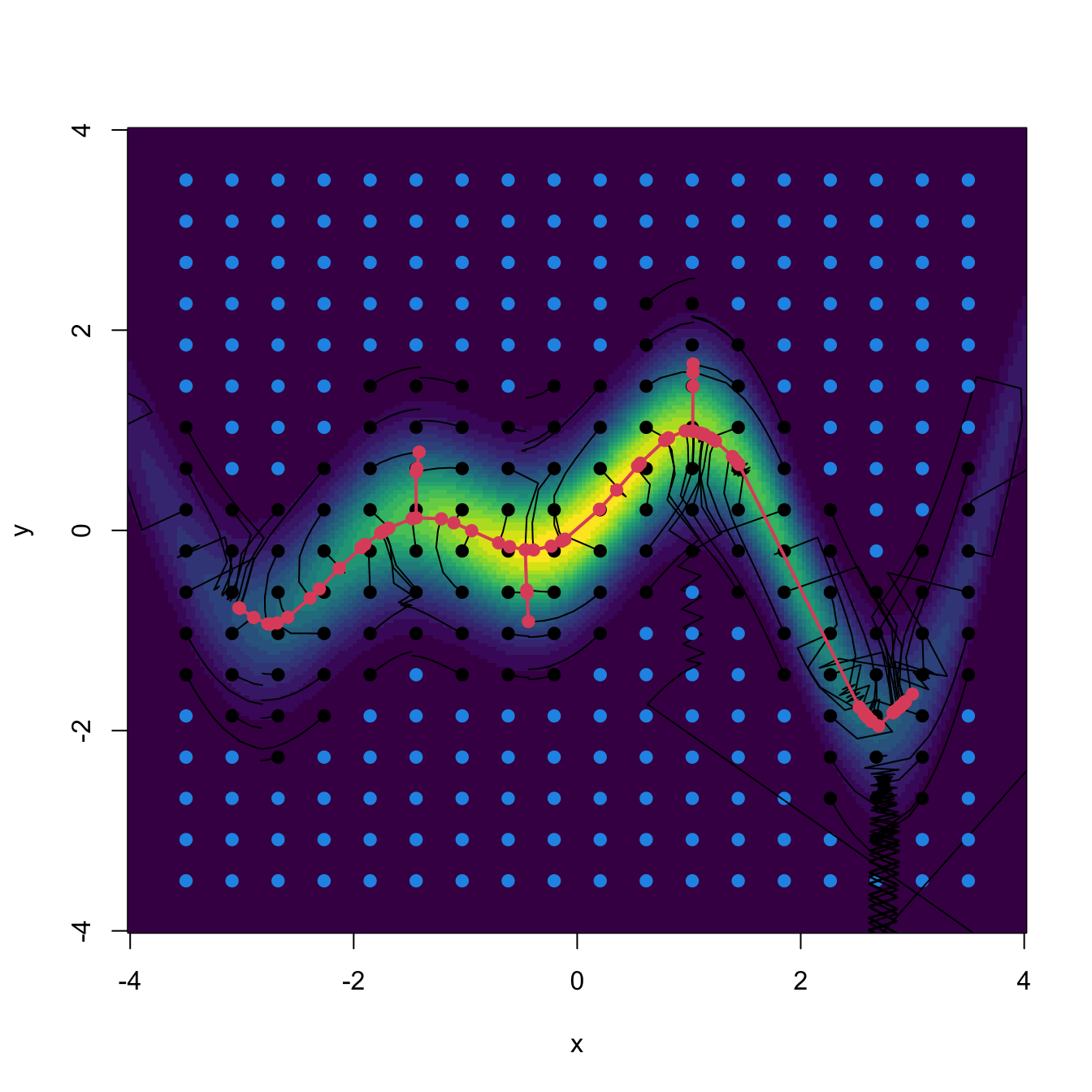
Figure 3.18: Highly non-normal densities and the construction of their density ridges. In blue, the points $\mathbf{x}_0$ that lie on low-density regions and are skipped from the Euler algorithm (longer running times and not useful output). In red, the final points $\mathbf{x}$ that lie on ridges on high-density regions (thus excluding ill-defined ridges). The red line is the Euclidean minimum spanning tree of the final points.

Exercise 3.31 Implement the Euler method for $f$ being f_oval, f_crois, and f_sin, in order to reproduce Figure 3.18. You will have to:

Implement the gradient and Hessian of $f.$ To avoid computing the analytical form, you can rely on numDeriv::grad and numDeriv::hessian to evaluate numerically $\mathrm{D}f$ and $\mathrm{H}f$ (although this will run slower than the analytical form).
Skip initial values $\mathbf{x}_0$ such that $f(\mathbf{x}_0)<\delta,$ so that the Euler method is not run for them. This saves computational time.
Stop the iteration in the Euler method if absolute or relative convergence is attained. Precisely, stop if $\|\mathbf{x}_{t+1} - \mathbf{x}_t\|_\infty<\varepsilon\,$¹¹⁴ or $\|\mathbf{x}_{t+1} - \mathbf{x}_t\|_\infty/\|\mathbf{x}_t\|_\infty<\varepsilon.$ This saves computational time.
Disregard final values $\mathbf{x}$ from the density ridge if $f(\mathbf{x})<50\delta.$ This avoids spurious solutions.
Join points automatically using the Euclidean minimum spanning tree algorithm.
Tune the selection of $h,$ $N,$ $\varepsilon,$ and $\delta.$ You can start with $h=0.25,$ $N=100,$ $\varepsilon=10^{-4},$ and $\delta=10^{-3}.$

Estimating density ridges

Once the population view of density ridges is clear, estimating density ridges from a sample is conceptually trivial: just replace $f$ in (3.36) with its kde $\hat{f}(\cdot;\mathbf{H})$ and then apply the two tweaks employed in kernel mean shift clustering (3.26): replace the gradient with the normalized gradient and the step $h$ by $\mathbf{H}.$ By doing so, it results

\[\begin{align} \mathbf{x}_{t+1}=\mathbf{x}_t+\mathbf{H}\hat{\boldsymbol{\eta}}_{(p-1)}(\mathbf{x}_t;\mathbf{H}),\quad \hat{\boldsymbol{\eta}}_{(p-1)}(\mathbf{x};\mathbf{H}):=\frac{\mathrm{D}_{(p-1)}\hat{f}(\mathbf{x};\mathbf{H})}{\hat{f}(\mathbf{x};\mathbf{H})},\tag{3.37} \end{align}\]

where

\[\begin{align} \mathrm{D}_{(p-1)}\hat{f}(\mathbf{x};\mathbf{H}):=\hat{\mathbf{U}}_{(p-1)}(\mathbf{x};\mathbf{H})\hat{\mathbf{U}}_{(p-1)}(\mathbf{x};\mathbf{H})'\mathrm{D}\hat{f}(\mathbf{x};\mathbf{H}) \end{align}\]

and $\hat{\mathbf{U}}_{(p-1)}(\mathbf{x};\mathbf{H})$ stems from the eigendecomposition of the estimated Hessian: $\mathrm{H}\hat{f}(\mathbf{x};\mathbf{H})=\hat{\mathbf{U}}(\mathbf{x};\mathbf{H})\hat{\boldsymbol{\Lambda}}(\mathbf{x};\mathbf{H})\hat{\mathbf{U}}(\mathbf{x};\mathbf{H})'.$

The recipe for estimating density ridges from a sample $\mathbf{X}_1,\ldots,\mathbf{X}_n$ is now simple:

Select a “suitable” bandwidth $\hat{\mathbf{H}}.$
For each grid element $\{\mathbf{x}_{0,1},\ldots,\mathbf{x}_{0,m}\},$ iterate the recurrence relation (3.37) “until convergence” to a given $\mathbf{x}_j,$ $j=1,\ldots,m.$ Skip this step for $\mathbf{x}_{0,j}$ such that $\hat{f}(\mathbf{x}_{0,j};\mathbf{H})$ is not larger than a “certain threshold”.¹¹⁵
Set $\hat{\mathcal{R}}_1(f):=\{\mathbf{x}_1,\ldots,\mathbf{x}_m\}.$

The kind of bandwidth selectors recommended are the ones designed for Hessian density estimation (see Sections 3.1 and 3.4), since (3.37) critically depends on adequately estimating the Hessian for computing the projection into its second eigenvector (see discussion in Section 6.3 in Chacón and Duong (2018)). These bandwidth selectors yield larger bandwidths than the ones designed for density estimation (and also density gradient estimation).

In addition, both the iteration “until convergence” and the “certain threshold” have to be evaluated in practice with adequate numerical tolerances. The function ks::kdr implements kernel density ridge estimation and automatically employs tested choices for numerical tolerances, convergence criteria, and other tuning parameters. The following chunk of code shows its basic use in the examples of the “oval”, “croissant”, and “sin” densities.

# Simulation from the "oval" density
r_oval <- function(n, mu = 2, sigma = 0.35, 
                   Sigma = rbind(c(1, -0.71), c(-0.71, 2))) {

  # Sampling in polar coordinates
  r <- rnorm(n = n, mean = mu, sd = sigma)
  theta <- runif(n, 0, 2 * pi)
  x <- r * cbind(cos(theta), sin(theta))

  # Data rotation
  Sigma_sqrt <- chol(Sigma)
  return(x %*% Sigma_sqrt)

}

# Simulation from the "croissant" density
r_crois <- function(n, mu = 2, sigma = 0.5, mu_theta = pi / 2, kappa = 1) {

  # Sampling in polar coordinates as conditional * marginal
  theta <- circular:::RvonmisesRad(n = n, mu = mu_theta, kappa = kappa)
  r <- rnorm(n = n, mean = mu, sd = sigma)
  x <- r * cbind(cos(theta), sin(theta))
  return(x)

}

# Simulation from the "sin" density
r_sin <- function(n, a = 0.5, b = 1.75, sigma_x = 2, sigma_y = 0.5) {

  # Sampling as conditional * marginal
  x <- rnorm(n = n, mean = 0, sd = sigma_x)
  y <- rnorm(n = n, mean = a * (1 + x) * sin(b * x), sd = sigma_y)
  return(cbind(x, y))

}

# Oval
set.seed(123456)
samp_oval <- r_oval(n = 1e3)
kdr_oval <- ks::kdr(x = samp_oval)
plot(samp_oval)
col <- rainbow(max(kdr_oval$end.points$segment))[kdr_oval$end.points$segment]
points(kdr_oval$end.points[, 1:2], col = col)
emst <- emstreeR::ComputeMST(x = kdr_oval$end.points[, 1:2], verbose = FALSE)
segments(x0 = kdr_oval$end.points[emst$from, 1],
         y0 = kdr_oval$end.points[emst$from, 2],
         x1 = kdr_oval$end.points[emst$to, 1],
         y1 = kdr_oval$end.points[emst$to, 2], lwd = 2)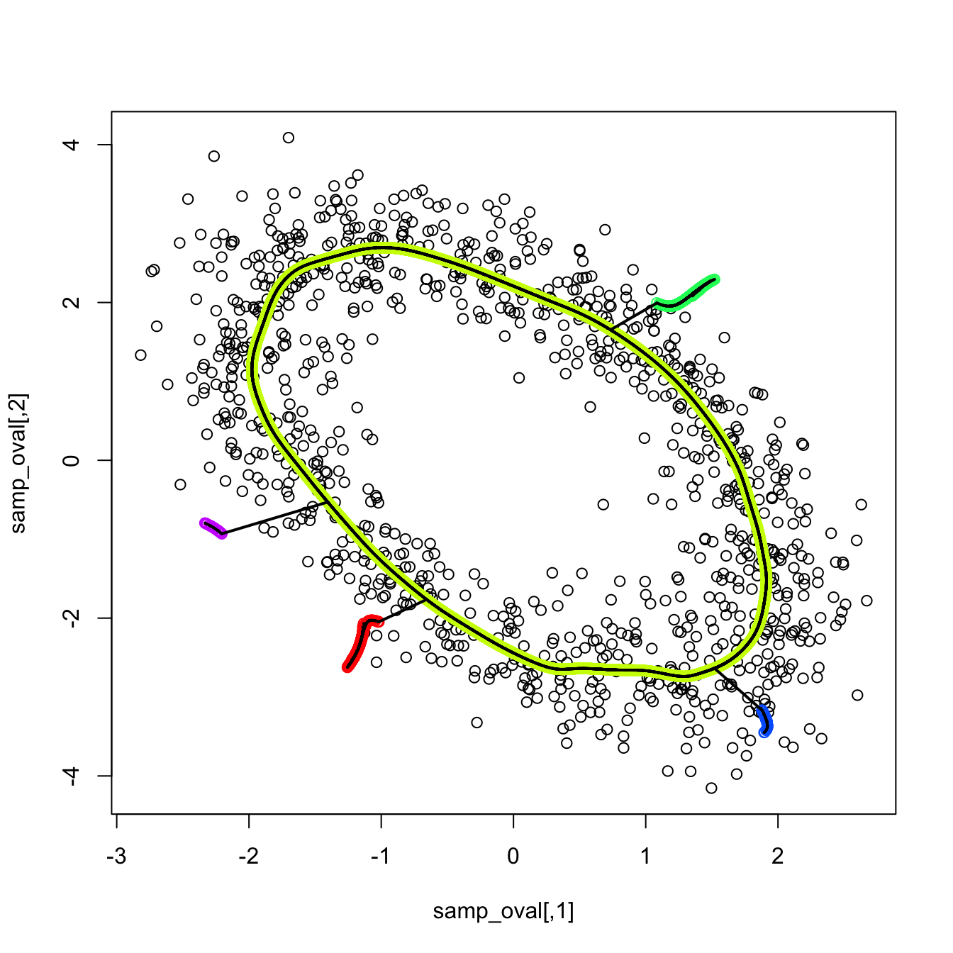

# The $end.points$segment output of ks::kdr is very useful, as it allows
# handling the components of the ridges easily

# Croissant
set.seed(526123)
samp_crois <- r_crois(n = 1e3)
kdr_crois <- ks::kdr(x = samp_crois)
plot(samp_crois)
col <- rainbow(max(kdr_crois$end.points$segment))[kdr_crois$end.points$segment]
points(kdr_crois$end.points[, 1:2], col = col)
emst <- emstreeR::ComputeMST(x = kdr_crois$end.points[, 1:2], verbose = FALSE)
segments(x0 = kdr_crois$end.points[emst$from, 1],
         y0 = kdr_crois$end.points[emst$from, 2],
         x1 = kdr_crois$end.points[emst$to, 1],
         y1 = kdr_crois$end.points[emst$to, 2], lwd = 2)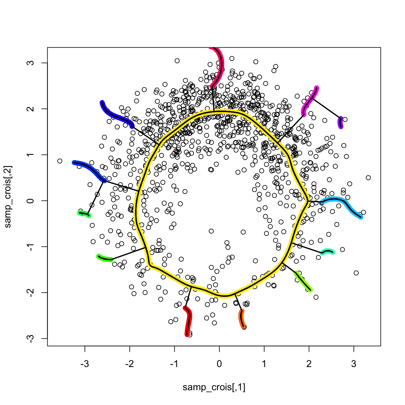


# Sin
set.seed(123456)
samp_sin <- r_sin(n = 1e3)
kdr_sin <- ks::kdr(x = samp_sin)
plot(samp_sin)
col <- rainbow(max(kdr_sin$end.points$segment))[kdr_sin$end.points$segment]
points(kdr_sin$end.points[, 1:2], col = col)
emst <- emstreeR::ComputeMST(x = kdr_sin$end.points[, 1:2], verbose = FALSE)
segments(x0 = kdr_sin$end.points[emst$from, 1],
         y0 = kdr_sin$end.points[emst$from, 2],
         x1 = kdr_sin$end.points[emst$to, 1],
         y1 = kdr_sin$end.points[emst$to, 2], lwd = 2)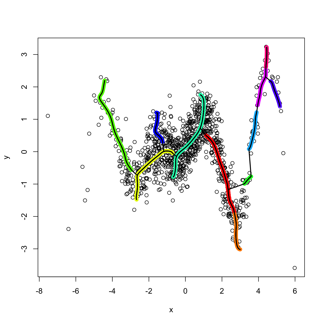

Further options of ks::kdr are described below.

# The initial values are chosen automatically, but they can be specified,
# gives faster computations
y <- expand.grid(seq(-3, 3, l = 20), seq(-4, 4, l = 20))

# Use y and save paths
kdr_oval_1 <- ks::kdr(x = samp_oval, y = y, keep.path = TRUE)
plot(samp_oval)
paths <- kdr_oval_1$path
points(kdr_oval_1$y, col = 4, pch = 19, cex = 0.5)
for (i in seq_along(paths)) {

  lines(paths[[i]], col = 4, cex = 0.5)

}
points(kdr_oval_1$end.points, col = 2, pch = 19)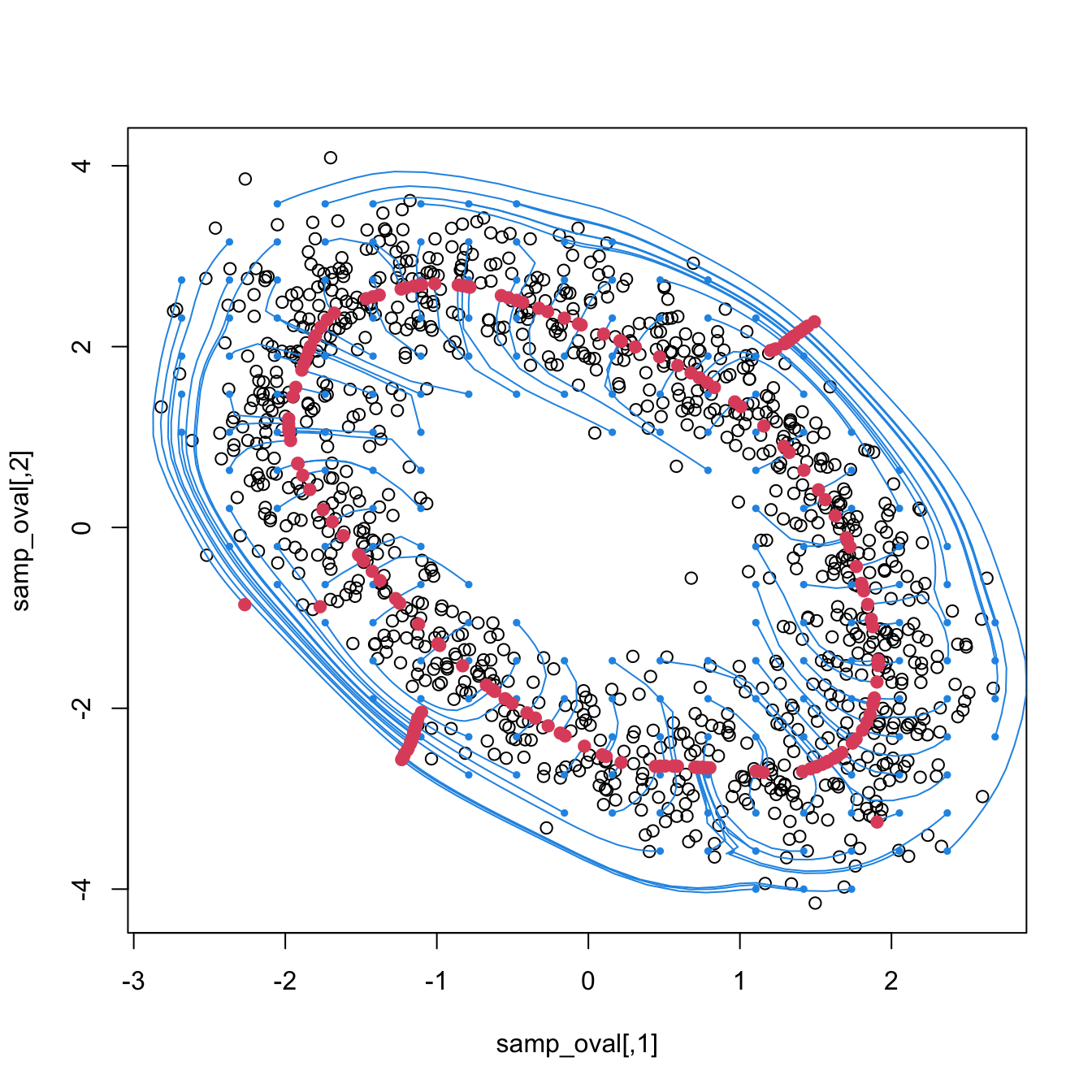

length(paths) # Ascent done only for 235 out of the 400 y's
## [1] 201

# By default, ks::kdr employs H = ks::Hpi(..., deriv.order = 2). It can be
# precomputed to reduce the computational cost of ks::kdr(). But care is needed:
# if H is provided, ks::kdr() needs to be called with pre = FALSE to avoid an
# internal scaling of the sample that will result in H being not adequate for
# the scaled sample
H <- ks::Hpi(x = samp_oval, deriv.order = 2)
kdr_oval_1a <- ks::kdr(x = samp_oval, H = H, pre = FALSE, keep.path = TRUE)

# There is a bug in ks 1.13.3 that prevents using pre = FALSE and y at the same
# time. A partial fix is to specify xmin/xmax and gridsize, which will determine
# y, but keeping in mind that these parameters will also affect the precision of
# the Hessian estimation (so if they are too small to save computing time, the
# accuracy of the ridge estimation will decrease)
kdr_oval_1b <- ks::kdr(x = samp_oval, H = H, xmin = c(-3, -4), xmax = c(3, 4),
                       gridsize = c(20, 20), pre = FALSE, keep.path = TRUE)

# Compare different approaches -- same main structure, different end points
# and spurious ridges depending on the size of the initial grid
plot(samp_oval, ylim = c(-4, 6))
points(kdr_oval_1a$end.points[, 1:2], col = 2, pch = 19, cex = 1)
points(kdr_oval_1b$end.points[, 1:2], col = 3, pch = 19, cex = 0.25)
points(kdr_oval_1$end.points[, 1:2], col = 4, pch = 19, cex = 0.25)
legend("topright", legend = c("H given, default y",
                              "xmin/xmax/gridsize/H given",
                              "y given, default H"), col = 2:4, lwd = 2)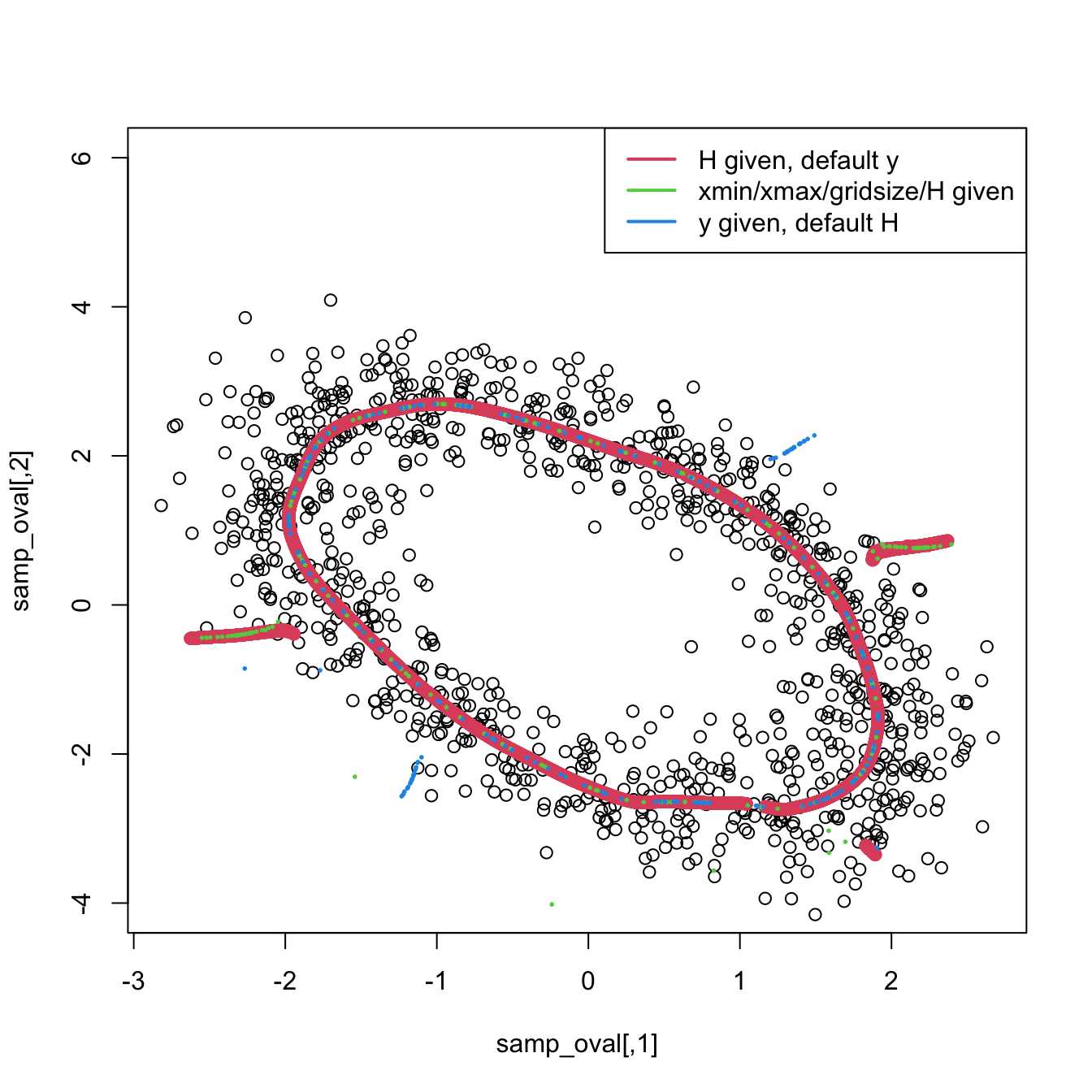

length(kdr_oval_1$path) # y given, default H
## [1] 201
length(kdr_oval_1a$path) # H given, default y
## [1] 9419
length(kdr_oval_1b$path) # xmin/xmax/gridsize/H given
## [1] 201

# If we want to get rid of the points outside the oval, we can identify
# them using the density level set for alpha = 0.15
plot(samp_oval)
points(kdr_oval_1$end.points, col = 2, pch = 19)
alpha <- 0.15
supp <- ks::ksupp(fhat = ks::kde(x = samp_oval, H = H),
                  cont = (1 - alpha) * 100, convex.hull = FALSE)
points(supp, col = 3, cex = 0.5)

# Two ways of excluding the "spurious" ridges: via convex hull and via
# fhat < c_alpha
C <- geometry::convhulln(p = supp)
out_chull <- !geometry::inhulln(ch = C, p =
                                  as.matrix(kdr_oval_1$end.points)[, 1:2])
c_alpha <- quantile(ks::kde(x = samp_oval, H = H,
                            eval.points = samp_oval)$estimate, probs = alpha)
out_kde <- ks::kde(x = samp_oval, H = H, eval.points =
                     kdr_oval_1$end.points[, 1:2])$estimate < c_alpha
points(kdr_oval_1$end.points[out_chull, 1:2], col = 4, cex = 0.75, pch = 19)
points(kdr_oval_1$end.points[out_kde, 1:2], col = 5, cex = 0.75, pch = 19)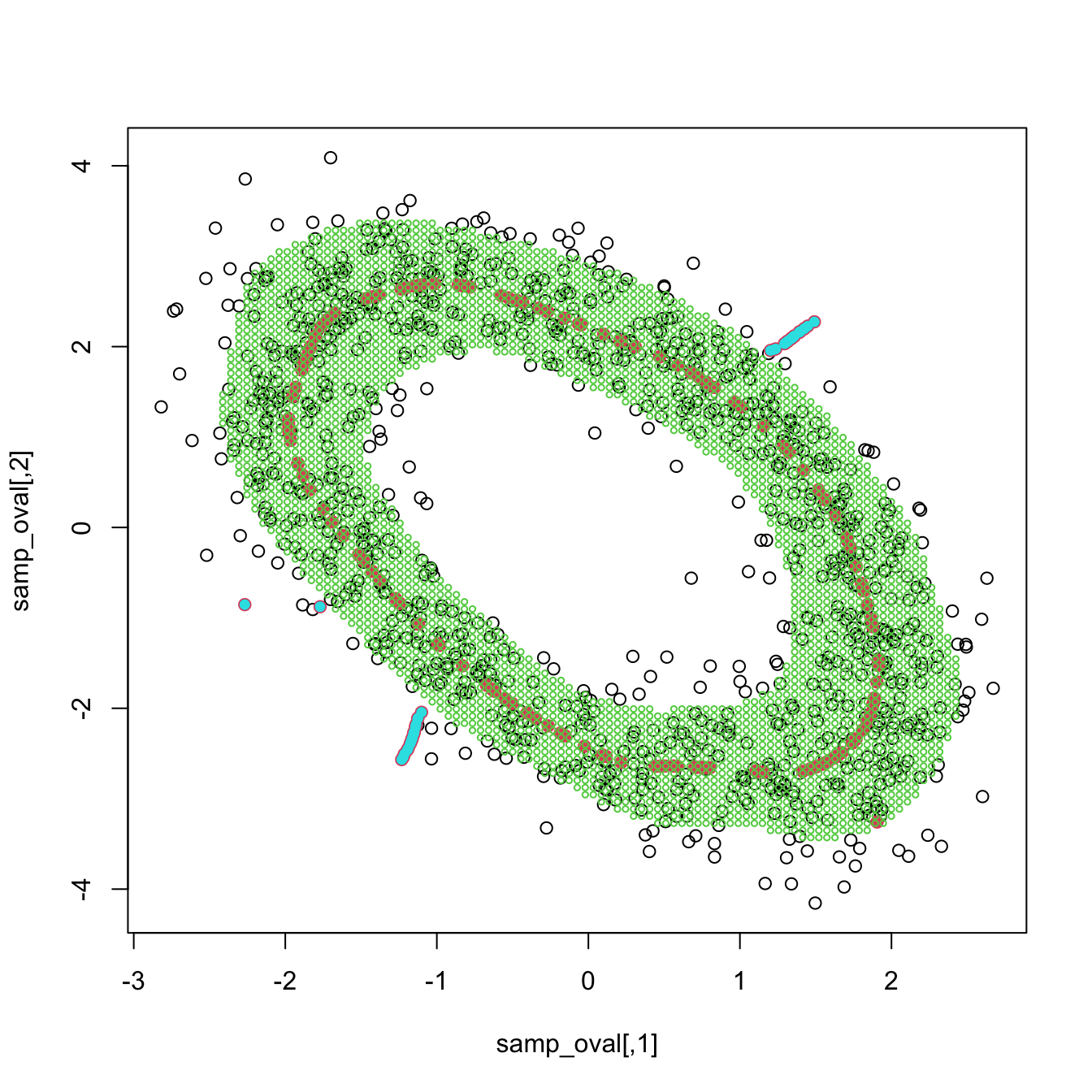


# The initial grid can also be specified with xmax, xmin, and gridsize
# (pre = FALSE because H is precomputed)
kdr_oval_2 <- ks::kdr(x = samp_oval, H = H, xmin = c(-3, -3), xmax = c(3, 3),
                      gridsize = c(20, 20), keep.path = TRUE, pre = FALSE)
plot(samp_oval)
points(kdr_oval_2$end.points[, 1:2], col = 2, pch = 19)
paths <- kdr_oval_2$path
points(kdr_oval_2$y, col = 4, pch = 19, cex = 0.5)
for (i in seq_along(paths)) {

  lines(paths[[i]], col = 4, cex = 0.5)

}


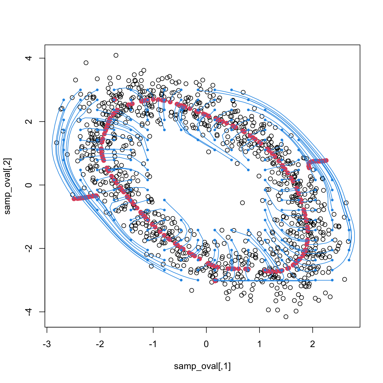
# Save also computing time by increasing density.cutoff
alpha <- 0.5
c_alpha <- quantile(ks::kde(x = samp_oval, H = H,
                            eval.points = samp_oval)$estimate, probs = alpha)
kdr_oval_3 <- ks::kdr(x = samp_oval, y = y, H = H, density.cutoff = c_alpha)
plot(samp_oval)
points(kdr_oval_3$y, col = 4, pch = 19, cex = 0.5)
points(kdr_oval_3$end.points[, 1:2], col = 2, pch = 19)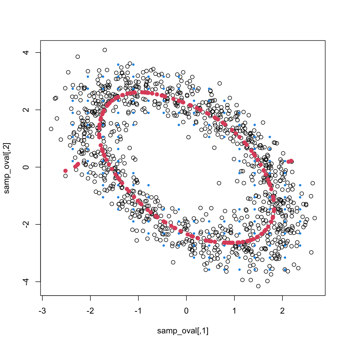

We conclude by showing a real data application of density ridges in the context of earthquakes. The snippet of code adapts the example in the documentation of ks::kdr.

# Load data
data(quake, package = "ks") # Earthquakes locations
data(plate, package = "ks") # Tectonic plate boundaries

# Select the Pacific Ring of Fire and disregard other variables
# except location of craters
quake <- quake[quake$prof == 1, c("long", "lat")]

# Fix negative longitude
quake$long[quake$long < 0] <- quake$long[quake$long < 0] + 360

# Select relevant plates
plate <- plate[plate$long < -20 | plate$long > 20, ]
plate$long[plate$long < 0 & !is.na(plate$long)] <-
  plate$long[plate$long < 0 & !is.na(plate$long)] + 360

# Display raw data
maps::map("world2", xlim = c(85, 305), ylim = c(-70, 70),
          mar = c(0, 0, 0, 0), interior = FALSE, lty = 2)
lines(plate[, 1:2], col = 3, lwd = 2)
points(quake, cex = 0.5, pch = 16, col = 2)

# Density ridges
kdr_quake <- ks::kdr(x = quake, xmin = c(70, -70), xmax = c(310, 80))
points(kdr_quake$end.points[, 1:2], cex = 0.5, pch = 16, col = 4)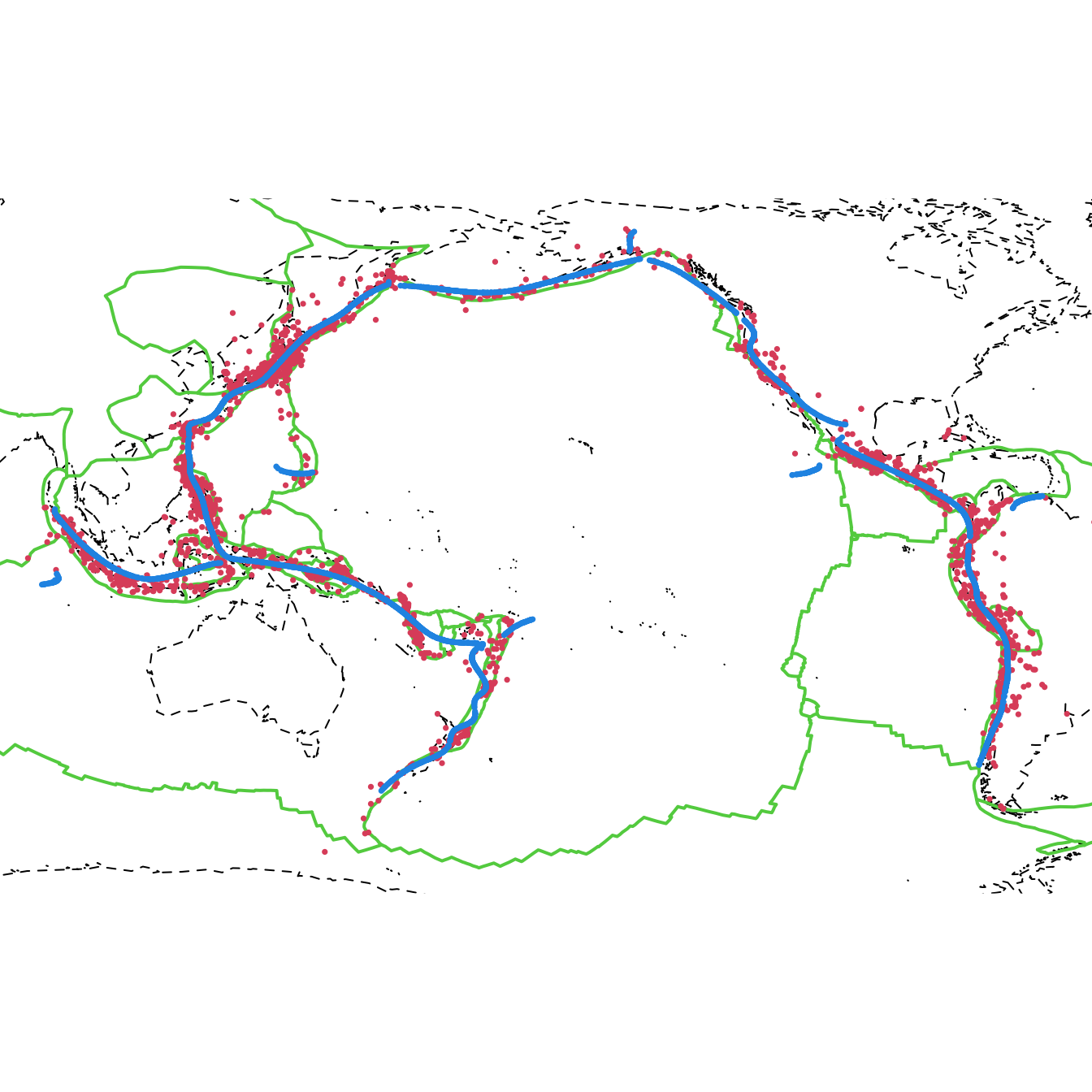

Estimated density ridges for the quake dataset. Observe how the density ridges (blue) of the earthquakes locations (red) reveal the relation between earthquakes and tectonic plate boundaries (green).

Figure 3.19: Estimated density ridges for the quake dataset. Observe how the density ridges (blue) of the earthquakes locations (red) reveal the relation between earthquakes and tectonic plate boundaries (green).

Exercise 3.32 Apply ks::kdr to the msds.RData dataset. Investigate the effect of different bandwidths selectors on the resulting estimated ridges trying $\hat{\mathbf{H}}_{\mathrm{NS},r}$ and $\hat{\mathbf{H}}_{\mathrm{PI},r},$ for $r=0,1,2.$ Beware! The dataset is large. You may want to precompute bandwidths (use pre = FALSE in ks::kdr() if H is supplied) and be careful on the selection of the initial grid. Are you able to reproduce the main features of the data? Which ones are easier to catch?

References

Benjamini, Y. 1988. “Opening the Box of a Boxplot.” The American Statistician 42 (4): 257–62. https://doi.org/10.1080/00031305.1988.10475580.

Chacón, J. E. 2015. “A Population Background for Nonparametric Density-Based Clustering.” Statistical Science 30 (4): 518–32. https://doi.org/10.1214/15-STS526.

Chacón, J. E., and T. Duong. 2018. Multivariate Kernel Smoothing and Its Applications. Vol. 160. Monographs on Statistics and Applied Probability. Boca Raton: CRC Press. https://doi.org/10.1201/9780429485572.

Cuesta-Albertos, J. A., A. Gordaliza, and C. Matrán. 1997. “Trimmed $k$-Means: An Attempt to Robustify Quantizers” 25 (2): 553–76. https://doi.org/10.1214/aos/1031833664.

Fukunaga, K., and L. D. Hostetler. 1975. “The Estimation of the Gradient of a Density Function, with Applications in Pattern Recognition.” IEEE Transactions on Information Theory 21 (1): 32–40. https://doi.org/10.1109/tit.1975.1055330.

Genovese, C. R., M. Perone-Pacifico, I. Verdinelli, and L. Wasserman. 2014. “Nonparametric Ridge Estimation.” The Annals of Statistics 42 (4): 1511–45. https://doi.org/10.1214/14-AOS1218.

Hintze, J. L., and R. D. Nelson. 1998. “Violin Plots: A Box Plot-Density Trace Synergism.” The American Statistician 52 (2): 181–84. https://doi.org/10.1080/00031305.1998.10480559.

James, G., D. Witten, T. Hastie, and R. Tibshirani. 2013. An Introduction to Statistical Learning. Vol. 103. Springer Texts in Statistics. New York: Springer. https://doi.org/10.1007/978-1-4614-7138-7.

Tukey, J. W. 1977. Exploratory Data Analysis. Behavioral Science: Quantitative Methods. Reading: Addison-Wesley Publishing Company.

van der Maaten, L., and G. Hinton. 2008. “Visualizing Data Using $t$-SNE.” Journal of Machine Learning Research 9 (86): 2579–2605. http://jmlr.org/papers/v9/vandermaaten08a.html.

Wickham, H., and L. Stryjewski. 2011. “40 Years of Boxplots.” https://vita.had.co.nz/papers/boxplots.pdf.

Such as, e.g., intervals in $\mathbb{R}.$↩︎
The kde is not exogenous to box plots. Several kde-based variants of box plots have been produced, such as the popular violin plots by Hintze and Nelson (1998); see Benjamini (1988) and Wickham and Stryjewski (2011).↩︎
The construction of the box plot by Tukey (1977) seems to be influenced by the normal distribution. For a $\mathcal{N}(0,\sigma^2),$ the “$1.5\times\mathrm{IQR}$ rule” that flags an observation as an outlier has a special interpretation. Since $1.5\times\mathrm{IQR}=1.5\times(\Phi^{-1}(0.75)-\Phi^{-1}(0.25))\sigma\approx2.0235\sigma,$ an observation is flagged as an outlier if it is below $\mathrm{Q1}-1.5\times\mathrm{IQR}=\Phi^{-1}(0.25)\sigma-2.0235\sigma\approx-2.6980\sigma$ or above $\mathrm{Q3}+1.5\times\mathrm{IQR}\approx2.6980\sigma.$ This is slightly more liberal than the “$3\sigma$ rule” that accounts for 99.73% of the probability, which seems too restrictive for outlier-hunting. Tukey’s $1.5\times\mathrm{IQR}$ rule precisely determines that 99.3% of the points are not outliers. The closeness of this percentage to $99\%$ might explain the magic behind the $1.5$ factor.↩︎
Which is based on the assumption that $\mathbf{X}\sim\mathcal{N}_p(\boldsymbol{\mu},\boldsymbol{\Sigma}).$↩︎
Which can be seen as a special case of fitting a mixture of $k$ normals with isotropic covariance matrices $\boldsymbol{\Sigma}=c\mathbf{I}_p,$ $c>0.$↩︎
The difference between LDA and QDA is that the former assumes $\boldsymbol{\Sigma}_1=\boldsymbol{\Sigma}_2$ when confronting $\mathcal{N}_p(\boldsymbol{\mu}_1,\boldsymbol{\Sigma}_1)$ against $\mathcal{N}_p(\boldsymbol{\mu}_2,\boldsymbol{\Sigma}_2),$ whereas the latter does not. As a consequence, LDA produces a separating hyperplane between both classes, whereas QDA produces a separating quadric surface (such as a hyperboloid or paraboloid in $\mathbb{R}^3$).↩︎
Indeed, the principal components can be regarded as the maximum likelihood estimators of the eigenvectors of $\boldsymbol{\Sigma}$ when $\mathbf{X}\sim\mathcal{N}_p(\boldsymbol{\mu},\boldsymbol{\Sigma}).$↩︎
Since $\int f(\mathbf{x})\,\mathrm{d}\mathbf{x}=1,$ the scale for a pdf $f$ decreases as the dimension $p$ increases, as the volume in $\mathbb{R}^p$ grows exponentially with $p.$↩︎
We consider the largest $c_\alpha$ such that $\int_{\mathcal{L}(f;c_\alpha)}f(\mathbf{x})\,\mathrm{d}\mathbf{x}\geq 1-\alpha,$ instead of the $c_\alpha$ such that $\int_{\mathcal{L}(f;c_\alpha)}f(\mathbf{x})\,\mathrm{d}\mathbf{x}=1-\alpha,$ because the function $c\in[0,\infty)\mapsto\int_{\mathcal{L}(f;c)}f(\mathbf{x})\,\mathrm{d}\mathbf{x}\in[0,1]$ may not be continuous: think about $f(x)=1_{\{0<x<1\}}$ and $c=1.$ What is $c_{\alpha}$ for $\alpha=1/2$ in this case?↩︎
Smallest in terms of volume in $\mathbb{R}^p.$ Since $f$ is measuring the density of probability per volume in $\mathbb{R}^p,$ the highest density regions minimize the amount of volume required for allocating at least $1-\alpha$ probability. If $p=1,$ then the union of intervals that conform $\mathcal{L}(f;c_\alpha)$ has the shortest length possible to allocate $1-\alpha$ probability.↩︎
Identifying outlying observations in $\mathbb{R}^p$ is much more challenging than in $\mathbb{R},$ and several statistical techniques have been proposed for that purpose. Indeed, the precise definition of what an outlier is in $\mathbb{R}^p$ admits several approaches. Here we just consider outliers as the points observed in low-density regions.↩︎
A set $C$ is convex in $\mathbb{R}^p$ if all the paths that interpolate two points $\mathbf{x},\mathbf{y}\in C$ are contained in $C.$ Mathematically, $C$ is convex if, for all $\mathbf{x},\mathbf{y}\in C,$ $t\mathbf{x}+(1-t)\mathbf{y}\in C,$ for all $t\in (0,1).$↩︎
Since version 0.4.0.↩︎
Obviously, the accuracy of this approximation depends on how convex is $\mathcal{L}(\hat{f}(\cdot;\mathbf{H});c).$↩︎
Computing $\hat{f}_i(\tilde{\mathbf{X}}_i;\hat{\mathbf{H}}_\mathrm{NS})$ for evaluating the outlyingness of $\tilde{\mathbf{X}}_i,$ rather than computing $\hat{f}(\tilde{\mathbf{X}};\hat{\mathbf{H}}_\mathrm{NS}),$ is important. In $\hat{f}_i(\tilde{\mathbf{X}}_i;\hat{\mathbf{H}}_\mathrm{NS}),$ the estimated density at $\tilde{\mathbf{X}}_i$ is computed with $\mathbf{X}_1,\ldots,\mathbf{X}_{n_1},\tilde{\mathbf{X}}_i,$ so “the contribution of $\tilde{\mathbf{X}}_i$ to itself”, $\frac{1}{n_1+1}K_{\hat{\mathbf{H}}_\mathrm{NS}}(\mathbf{0}),$ is present in the kde. Which is exactly the same situation that happens when computing $\hat{f}(\mathbf{X}_1;\hat{\mathbf{H}}_\mathrm{NS}),\ldots,\hat{f}(\mathbf{X}_{n_1};\hat{\mathbf{H}}_\mathrm{NS})$ for estimating $\hat c_\alpha,$ and so the comparison $\hat{f}_i(\tilde{\mathbf{X}}_i;\hat{\mathbf{H}}_\mathrm{NS})<\hat{c}_\alpha$ is “fair”.↩︎
Notice that $W(C_j)$ can be seen as the sample variance, since $W(C_j)=\frac{1}{|C_j|}\sum_{i,i'\in C_j} \|\mathbf{X}_i-\bar{\mathbf{X}}_{C_j}+\bar{\mathbf{X}}_{C_j}-\mathbf{X}_{i'}\|^2=\frac{2}{|C_j|}\sum_{i\in C_j} \|\mathbf{X}_i-\bar{\mathbf{X}}_{C_j}\|^2,$ where $\bar{\mathbf{X}}_{C_j}:=\frac{1}{|C_j|}\sum_{i\in C_j}\mathbf{X}_i$ is the sample mean of the observations in $C_j.$ Therefore, $W(C_j)=2S^2_{C_j},$ where $S^2_{C_j}$ is the trace of the sample covariance matrix $\frac{1}{|C_j|}\sum_{i\in C_j} (\mathbf{X}_i-\bar{\mathbf{X}}_{C_j})(\mathbf{X}_i-\bar{\mathbf{X}}_{C_j})'.$↩︎
It is possible to build a population formulation of $k$-means. That can be seen, e.g., in Cuesta-Albertos, Gordaliza, and Matrán (1997), a paper that introduces a trimmed variant of $k$-means.↩︎
The population view of $k$-means is conceptually more involved and less insightful than, as seen subsequently, mode clustering. The latter has an elegant simple connection with the (population) concept of mode.↩︎
For example, what are the clusters of the “claw” density nor1mix::MW.nm10?↩︎
Which is the right amount of clusters for the “claw” density?↩︎
Technically, excluding sets of zero Lebesgue measure.↩︎
The superscript $s$ stands for stable manifold and the subscript $+$ emphasizes that the positive gradient is considered.↩︎
Notice that (3.22) forces the derivative of $\boldsymbol{\phi}_{\mathbf{x}}$ at $t$ to coincide with the gradient of $f$ at $\boldsymbol{\phi}_{\mathbf{x}}(t).$↩︎
Observe that the iterative scheme will converge to a stationary point when $\mathrm{D}f(\mathbf{x}_t)\approx0,$ that is, when $\mathbf{x}_t$ approaches $\boldsymbol{\xi}$ such that $\mathrm{D}f(\boldsymbol{\xi})=0.$↩︎
Recall: once the population setting is well-defined, the sample version becomes immediately clear.↩︎
Both inspired by the original mean shift recurrence relation proposed by Fukunaga and Hostetler (1975).↩︎
Notice that, on the one hand, the normalized gradient is automatically magnified if the density at $\mathbf{x}$ is low, avoiding very slow movements in low-density regions. On the other hand, the normalizing gradient is decreased automatically at high-density regions, avoiding the “overshooting” of the local maximum.↩︎
Because it can be seen that a factor $\mathbf{H}^{-1}$ appears in the expansion of $\hat{\boldsymbol{\eta}}(\mathbf{x}_t;\mathbf{H})$ after taking derivatives, a factor that is canceled when premultiplied by $\mathbf{H}$ if $\mathbf{A}=\mathbf{H}.$↩︎
Observe that this is key to determine how many different modes, therefore clusters, the algorithm has found.↩︎
This is a very appealing benefit of kernel mean shift clustering that is not possible in a principled form in other clustering methods.↩︎
Observe that, since we are interested in the argument $j$ that maximizes $\mathbb{P}[Y=j|\mathbf{X}=\mathbf{x}],$ we do not care about the standardization by $\sum_{j=1}^m \pi_jf_j(\mathbf{x})$ in (3.28), as this is a constant common factor for all $j=1,\ldots,m.$↩︎
Notice that one could also choose $\mathbf{H}_j,$ $j=1,\ldots,m,$ to maximize classification accuracy directly, rather than to estimate accurately $f_j,$ $j=1,\ldots,m.$ This would be a more complicated procedure, though, as it will involve optimizing a classification criterion over $(\mathrm{vech}(\mathbf{H}_1)',\ldots,\mathrm{vech}(\mathbf{H}_m)')'\in\mathbb{R}^{mp(p-1)/2},$ as opposed to select $m$ bandwidth matrices separately. As $\mathrm{vec},$ the $\mathrm{vech}$ operator stacks the columns of any matrix into a long vector, but $\mathrm{vech}$ first removes the lower diagonal matrix.↩︎
Meaning that its expectation $\boldsymbol{\mu}$ is zero. Otherwise, the principal directions given in $\mathbf{U}$ and corresponding to $\{c\mathbf{u}_i:c\in\mathbb{R}\},$ $i=1,\ldots,p,$ need to be shifted by $\boldsymbol{\mu},$ i.e., $\{\boldsymbol{\mu}+c\mathbf{u}_i:c\in\mathbb{R}\},$ $i=1,\ldots,p,$ which is inconvenient. This requirement is not restrictive, as it is trivial to center a random vector and a sample.↩︎
Because the moment and maximum likelihood estimators for $(\boldsymbol{\mu},\boldsymbol{\Sigma})$ in $\mathcal{N}_p(\boldsymbol{\mu},\boldsymbol{\Sigma})$ coincide.↩︎
Compare it, e.g., with a zig-zagged ascending path: the rate of change of its slope varies significantly at its bends.↩︎
A long, narrow raised part of a surface, especially a high edge along a mountain.↩︎
Curvature can be positive or negative!↩︎
Because $\mathbf{U}(\mathbf{x})$ is an orthogonal matrix.↩︎
Observe that the “maximum curvature” is understood in a signed form, and not in an absolute form. That is, $1$ is a larger signed curvature than $-3$.↩︎
Additionally, this removes the necessity of computing complicated normalizing constants for $f,$ as they will cancel out in the normalized gradient.↩︎
Can you imagine what the PC1 description of such densities would be?↩︎
$\|\mathbf{x}\|_\infty:=\max_{1\leq j\leq p}|x_j|.$↩︎
For example, run the step only if $\mathbf{x}_{0,j}\in\mathcal{L}(\hat{f}(\cdot;\mathbf{H});\hat{c}_\alpha),$ for $\alpha$ close to zero.↩︎