2.6 Kernel density estimation with ks
The density function in R presents certain limitations, such as the impossibility of evaluating the kde at arbitrary points, the unavailability of built-in transformations, and the lack of a multivariate extension. The ks package (Duong 2020) delivers the ks::kde function, providing these and other functionalities. It will be the workhorse for carrying out multivariate kde (Section 3.1). The only drawback of ks::kde to be aware of is that it only considers normal kernels – though these are by far the most popular.
The following chunk of code shows that density and ks::kde give the same outputs. It also presents some of the extra flexibility on the evaluation that ks::kde provides.
# Sample
n <- 5
set.seed(123456)
samp_t <- rt(n, df = 2)

# Comparison: same output and same parametrization for bandwidth
bw <- 0.75
plot(kde <- ks::kde(x = samp_t, h = bw), lwd = 3) # ?ks::plot.kde for options
lines(density(x = samp_t, bw = bw), col = 2)
# Beware: there is no lines() method for ks::kde objects

# The default h is the DPI obtained by ks::hpi
kde <- ks::kde(x = samp_t)

# Manual plot -- recall $eval.points and $estimate
lines(kde$eval.points, kde$estimate, col = 4)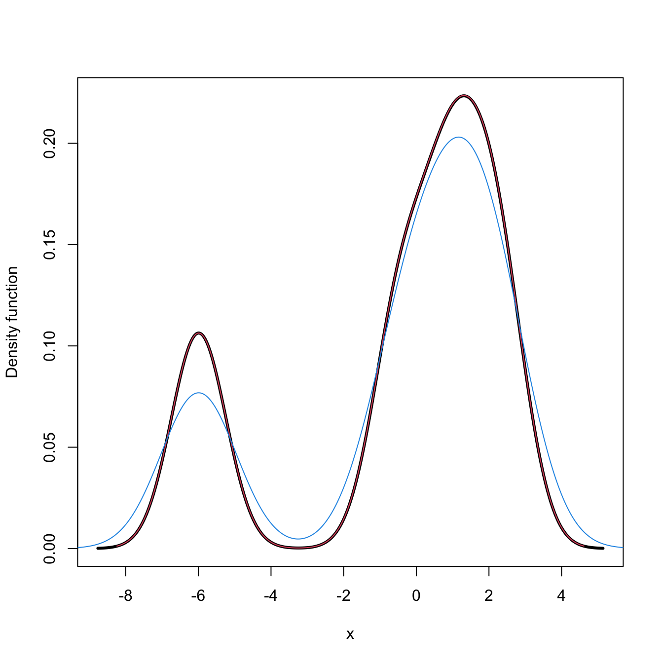
# Evaluating the kde at specific points, e.g., the first 2 sample points
ks::kde(x = samp_t, h = bw, eval.points = samp_t[1:2])
## $x
## [1]  1.4650470 -0.4971902  0.6701367  2.3647267 -5.9918352
##
## $eval.points
## [1]  1.4650470 -0.4971902
##
## $estimate
## [1] 0.2223029 0.1416113
##
## $h
## [1] 0.75
##
## $H
## [1] 0.5625
##
## $gridtype
## [1] "linear"
##
## $gridded
## [1] TRUE
##
## $binned
## [1] TRUE
##
## $names
## [1] "x"
##
## $w
## [1] 1 1 1 1 1
##
## $type
## [1] "kde"
##
## attr(,"class")
## [1] "kde"

# By default ks::kde() computes the *binned* kde (much faster) and then employs
# an interpolation to evaluate the kde at the given grid; if the exact kde is
# desired, this can be specified with binned = FALSE
ks::kde(x = samp_t, h = bw, eval.points = samp_t[1:2], binned = FALSE)
## $x
## [1]  1.4650470 -0.4971902  0.6701367  2.3647267 -5.9918352
##
## $eval.points
## [1]  1.4650470 -0.4971902
##
## $estimate
## [1] 0.2223316 0.1416132
##
## $h
## [1] 0.75
##
## $H
## [1] 0.5625
##
## $gridded
## [1] FALSE
##
## $binned
## [1] FALSE
##
## $names
## [1] "x"
##
## $w
## [1] 1 1 1 1 1
##
## $type
## [1] "kde"
##
## attr(,"class")
## [1] "kde"

# Changing the size of the evaluation grid
length(ks::kde(x = samp_t, h = bw, gridsize = 1e3)$estimate)
## [1] 1000
The computation of log-transformed kde is straightforward using the positive and adj.positive.
# Sample from a LN(0, 1)
set.seed(123456)
samp_ln <- rlnorm(n = 200)

# Log-kde without shifting
a <- seq(0.1, 2, by = 0.4) # Sequence of shifts
col <- viridis::viridis(length(a) + 1)
plot(ks::kde(x = samp_ln, positive = TRUE), col = col[1],
     main = "Log-transformed kde and the effect of adj.positive",
     xlim = c(0, 7.5), ylim = c(0, 0.75))
# If h is not provided, then ks::hpi() is called on the transformed data

# Shifting: larger a increases the bias
for (i in seq_along(a)) {
  plot(ks::kde(x = samp_ln, positive = TRUE, adj.positive = a[i]),
       add = TRUE, col = col[i + 1])
}
curve(dlnorm(x), col = 2, add = TRUE, n = 500)
rug(samp_ln)
legend("topright", legend = c("True density", paste("adj.positive =", c(0, a))),
       col = c(2, col), lwd = 2)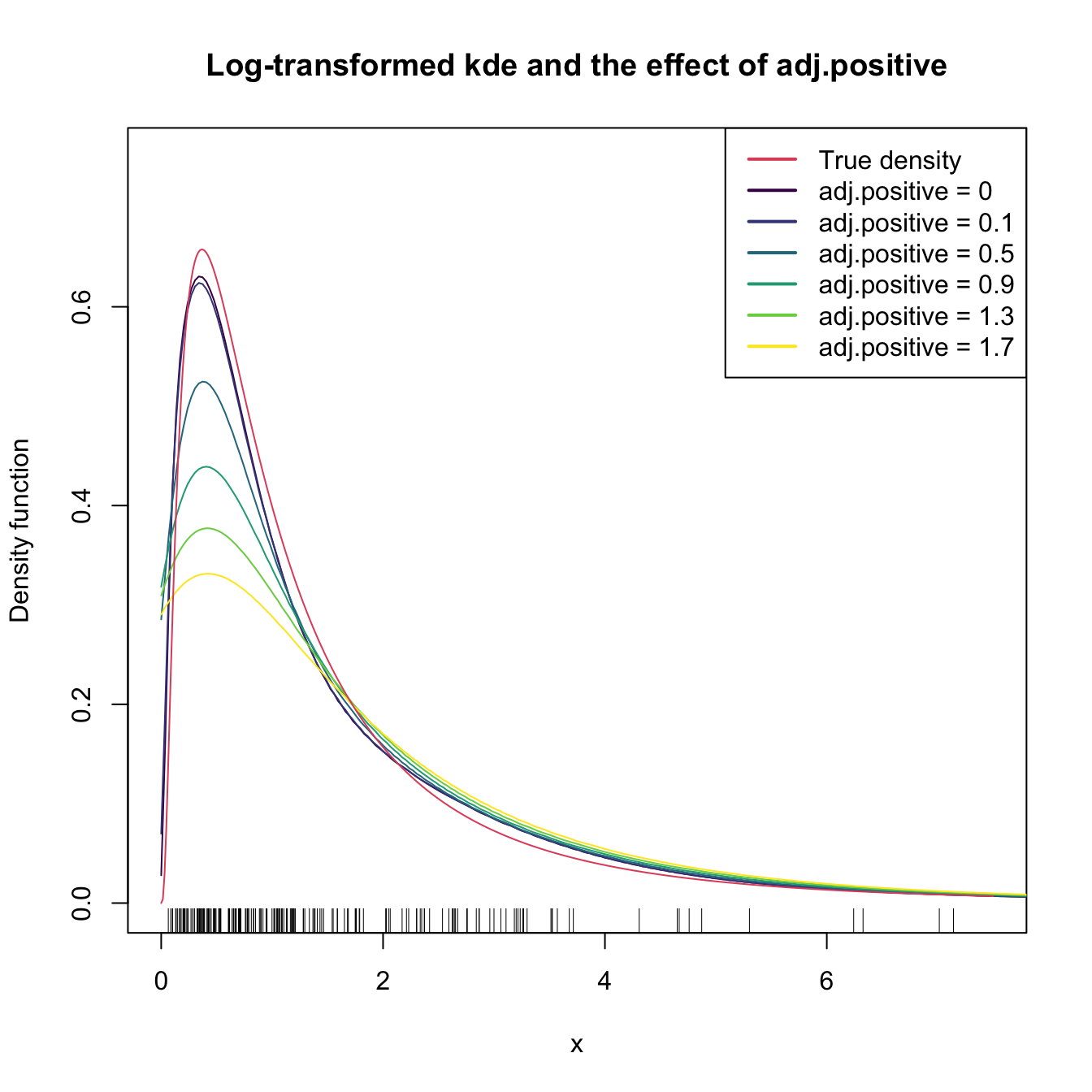
Finally, sampling from the kde and log-transformed kde is easily achieved by the use of ks::rkde.
# Untransformed kde
plot(kde <- ks::kde(x = log(samp_ln)), col = 4)
samp_kde <- ks::rkde(n = 5e4, fhat = kde)
plot(ks::kde(x = samp_kde), add = TRUE, col = 3)
legend("topright", legend = c("Kde", "Kde of sampled kde"),
       lwd = 2, col = 3:4)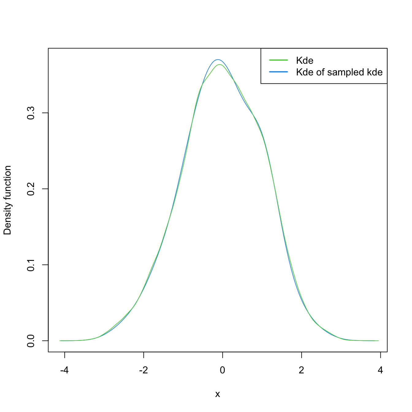
# Transformed kde
plot(kde_transf <- ks::kde(x = samp_ln, positive = TRUE), col = 4)
samp_kde_transf <- ks::rkde(n = 5e4, fhat = kde_transf, positive = TRUE)
plot(ks::kde(x = samp_kde_transf), add = TRUE, col = 3)
legend("topright", legend = c("Kde", "Kde of sampled kde"),
       lwd = 2, col = 3:4)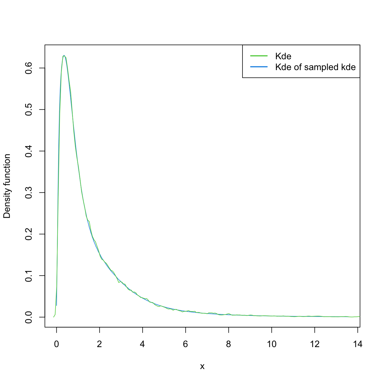
Exercise 2.25 Consider the MNIST dataset in the MNIST-tSNE.RData file. It contains the first \(60,000\) images of the MNIST database. Each observation is a grayscale image made of \(28\times 28\) pixels that is recorded as a vector of length \(28^2=784\) by concatenating the pixel columns. The entries of these vectors are numbers in \([0,1]\) indicating the level of grayness of the pixel: \(0\) for white, \(1\) for black. These vectorised images are stored in the \(60,000\times 784\) matrix in MNIST$x. The \(0\)–\(9\) labels of the digits are stored in MNIST$labels.
- Compute the average gray level,
av_gray_one, for each image of the digit “1”. - Compute and plot the kde of
av_gray_one. Consider taking into account that it is a positive variable. - Overlay the lognormal distribution density, with parameters estimated by maximum likelihood (use
MASS::fitdistr). - Repeat part c for the Weibull density.
- Which parametric model seems more adequate?