4.5 Kernel regression estimation with np | Notes for Nonparametric Statistics

4.5 Kernel regression estimation with `np`

The np package (Hayfield and Racine 2008) provides a complete framework for performing a more sophisticated nonparametric regression estimation for local constant and linear estimators, and for computing cross-validation bandwidths. The two workhorse functions for these tasks are np::npreg and np::npregbw, which they illustrate the philosophy behind the np package: first, a suitable bandwidth for the nonparametric method is found (via np::npregbw) and stored in an rbandwidth object; then, a fitting function (np::npreg) is called on that rbandwidth object, which contains all the needed information.

# Data -- nonlinear trend
data(Auto, package = "ISLR")
X <- Auto$weight
Y <- Auto$mpg

# np::npregbw computes by default the least squares CV bandwidth associated
# with a local *constant* fit and admits a formula interface (to be exploited
# more in multivariate regression)
bw0 <- np::npregbw(formula = Y ~ X)
## 
Multistart 1 of 1 |
Multistart 1 of 1 |
Multistart 1 of 1 |
Multistart 1 of 1 /
Multistart 1 of 1 |
Multistart 1 of 1 |
                   

# The spinner can be omitted with
options(np.messages = FALSE)

# Multiple initial points can be employed for minimizing the CV function (for
# one predictor, defaults to 1) and avoiding local minima
bw0 <- np::npregbw(formula = Y ~ X, nmulti = 2)

# The "rbandwidth" object contains useful information, see ?np::npregbw for
# all the returned objects
bw0
## 
## Regression Data (392 observations, 1 variable(s)):
## 
##                      X
## Bandwidth(s): 110.1476
## 
## Regression Type: Local-Constant
## Bandwidth Selection Method: Least Squares Cross-Validation
## Formula: Y ~ X
## Bandwidth Type: Fixed
## Objective Function Value: 17.66388 (achieved on multistart 2)
## 
## Continuous Kernel Type: Second-Order Gaussian
## No. Continuous Explanatory Vars.: 1
head(bw0)
## $bw
## [1] 110.1476
## 
## $regtype
## [1] "lc"
## 
## $pregtype
## [1] "Local-Constant"
## 
## $method
## [1] "cv.ls"
## 
## $pmethod
## [1] "Least Squares Cross-Validation"
## 
## $fval
## [1] 17.66388
# Recall that the fit is very similar to h_CV

# Once the bandwidth is estimated, np::npreg can be directly called with the
# "rbandwidth" object (it encodes the regression to be made, the data, the kind
# of estimator considered, etc). The hard work goes on np::npregbw, not on
# np::npreg
kre0 <- np::npreg(bws = bw0)
kre0
## 
## Regression Data: 392 training points, in 1 variable(s)
##                      X
## Bandwidth(s): 110.1476
## 
## Kernel Regression Estimator: Local-Constant
## Bandwidth Type: Fixed
## 
## Continuous Kernel Type: Second-Order Gaussian
## No. Continuous Explanatory Vars.: 1

# Plot directly the fit via plot() -- it employs as evaluation points the
# (unsorted!) sample
plot(kre0, col = 2, type = "o")
points(X, Y)
rug(X, side = 1); rug(Y, side = 2)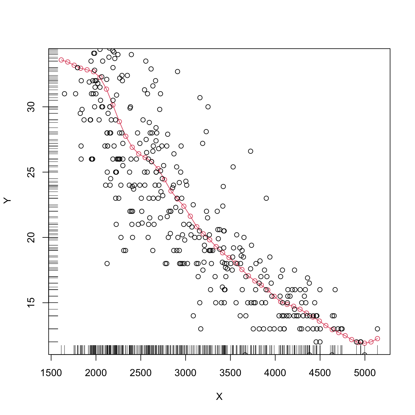

# lines(kre0$eval$X, kre0$mean, col = 3)

The type of local regression (local constant or local linear – no further local polynomial fits are implemented) is controlled by the argument regtype in np::npregbw: regtype = "ll" stands for “local linear” and regtype = "lc" for “local constant”.

# Local linear fit -- find first the CV bandwidth
bw1 <- np::npregbw(formula = Y ~ X, regtype = "ll")

# Fit
kre1 <- np::npreg(bws = bw1)

# Plot
plot(kre1, col = 2, type = "o")
points(X, Y)
rug(X, side = 1); rug(Y, side = 2)

The following code shows in more detail the output object associated with np::npreg and how to change the evaluation points.

# Summary of the npregression object
summary(kre0)
## 
## Regression Data: 392 training points, in 1 variable(s)
##                      X
## Bandwidth(s): 110.1476
## 
## Kernel Regression Estimator: Local-Constant
## Bandwidth Type: Fixed
## Residual standard error: 4.10312
## R-squared: 0.7230723
## 
## Continuous Kernel Type: Second-Order Gaussian
## No. Continuous Explanatory Vars.: 1

# Evaluation points (a data.frame) -- by default the sample (unsorted!)
head(kre0$eval)
##      X
## 1 3504
## 2 3693
## 3 3436
## 4 3433
## 5 3449
## 6 4341

# The estimation of the regression function at the evaluation points
head(kre0$mean)
## [1] 18.35364 17.10311 18.70083 18.71652 18.63411 14.23660

# The evaluation points can be changed using "exdat"
x_grid <- seq(1000, 5500, by = 5)
kre0 <- np::npreg(bws = bw0, exdat = x_grid)
kre1 <- np::npreg(bws = bw1, exdat = x_grid)

# Notice how $eval is a data.frame containing x_grid
head(kre0$eval)
##   x_grid
## 1   1000
## 2   1005
## 3   1010
## 4   1015
## 5   1020
## 6   1025

# This allows to compare estimators in a more transparent form
plot(X, Y)
lines(kre0$eval$x_grid, kre0$mean, col = 2)
lines(kre1$eval$x_grid, kre1$mean, col = 3)
rug(X, side = 1); rug(Y, side = 2)
legend("top", legend = c("Nadaraya-Watson", "Local linear"),
       lwd = 2, col = 2:3)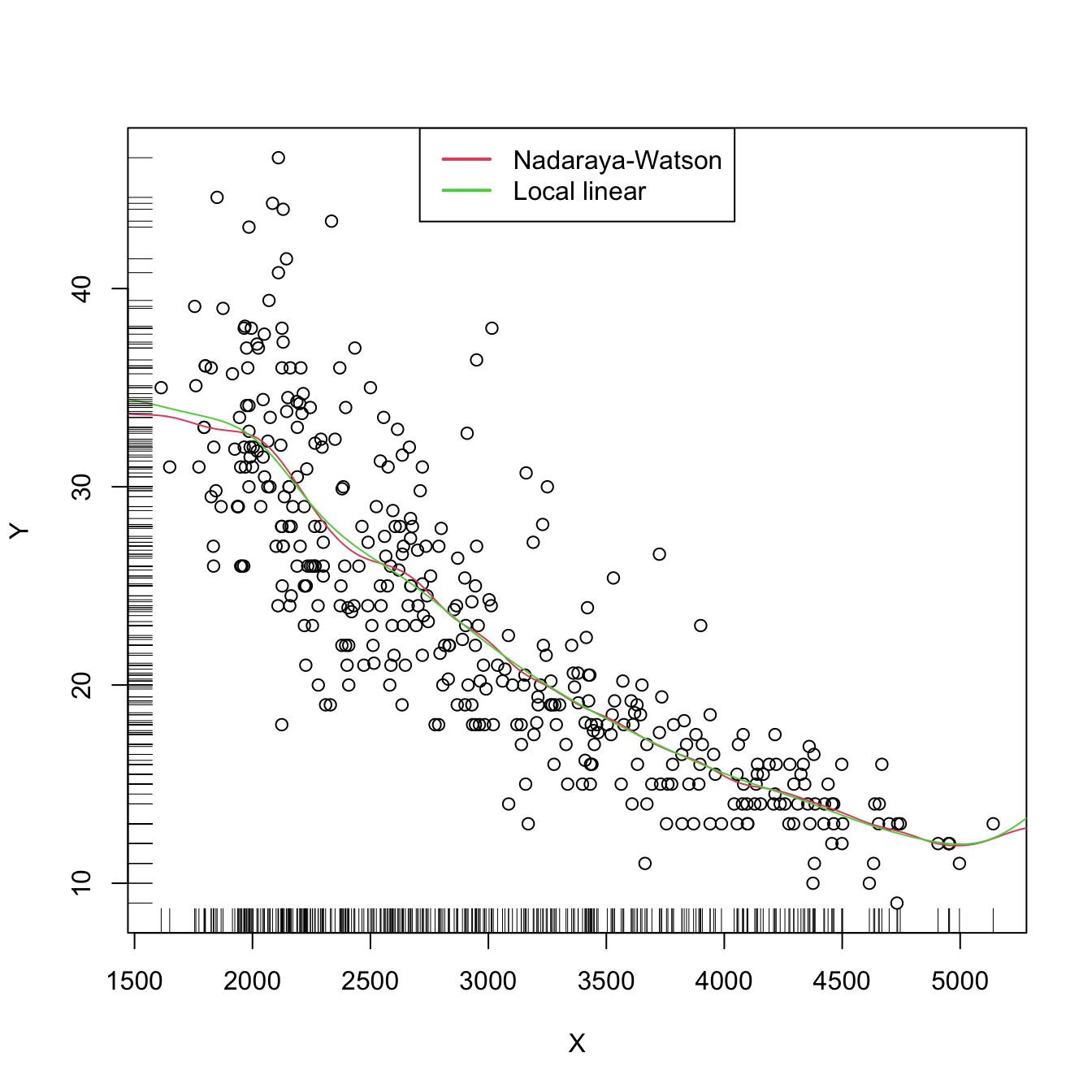

Now that we know how to effectively compute local constant and linear estimators, two insights with practical relevance become apparent:

The adequate bandwidths for the local linear estimator are usually larger than the adequate bandwidths for the local constant estimator. The reason is the extra flexibility that $\hat{m}(\cdot;1,h)$ has, which allows faster adaptation to variations in $m,$ whereas $\hat{m}(\cdot;0,h)$ can achieve this adaptability only by shrinking the neighborhood about $x$ by means of a smaller $h.$
Both estimators behave erratically at regions with low predictor’s density. This includes possible “holes” in the support of $X.$ In the absence of close data, the local constant estimator interpolates to a constant function that takes the value $Y_i$ of the closest $X_i$ to $x.$ However, the local linear estimator $\hat{m}(x;1,h)$ takes the value of the local linear regression $\hat{\beta}_{h,0}+\hat{\beta}_{h,1}(\cdot-x)$ that is determined by the two observations $(X_i,Y_i)$ with the closest $X_i$’s to $x.$ Hence, the local linear estimator extrapolates a line at regions with low $X$-density. This may have the undesirable consequence of yielding large spikes at these regions, which sharply contrasts with the “conservative behavior” of the local constant estimator.

The next two exercises are meant to evidence these two insights.

Exercise 4.18 Perform the following simulation study:

Simulate $n=100$ observations from the regression model $Y=m(X)+\varepsilon,$ where $X$ is distributed according to a nor1mix::MW.nm2, $m(x)=x\cos(x),$ and $\varepsilon+1\sim\mathrm{Exp}(1).$
Compute the CV bandwidths for the local constant and linear estimators.
Repeat Steps 1–2 $M=1,000$ times. Trick: use txtProgressBar() and setTxtProgressBar to have an indication of the progress of the simulation.

Compare graphically the two samples of CV bandwidths. To do so, show in a plot the log-transformed kdes for the two samples and imitate the display given in 4.5.

Estimated density for the local constant and local linear CV bandwidths, for the setting described in Exercise 4.18. The vertical bars denote the median CV bandwidths. Observe how local linear bandwidths tend to be larger than local constant ones.

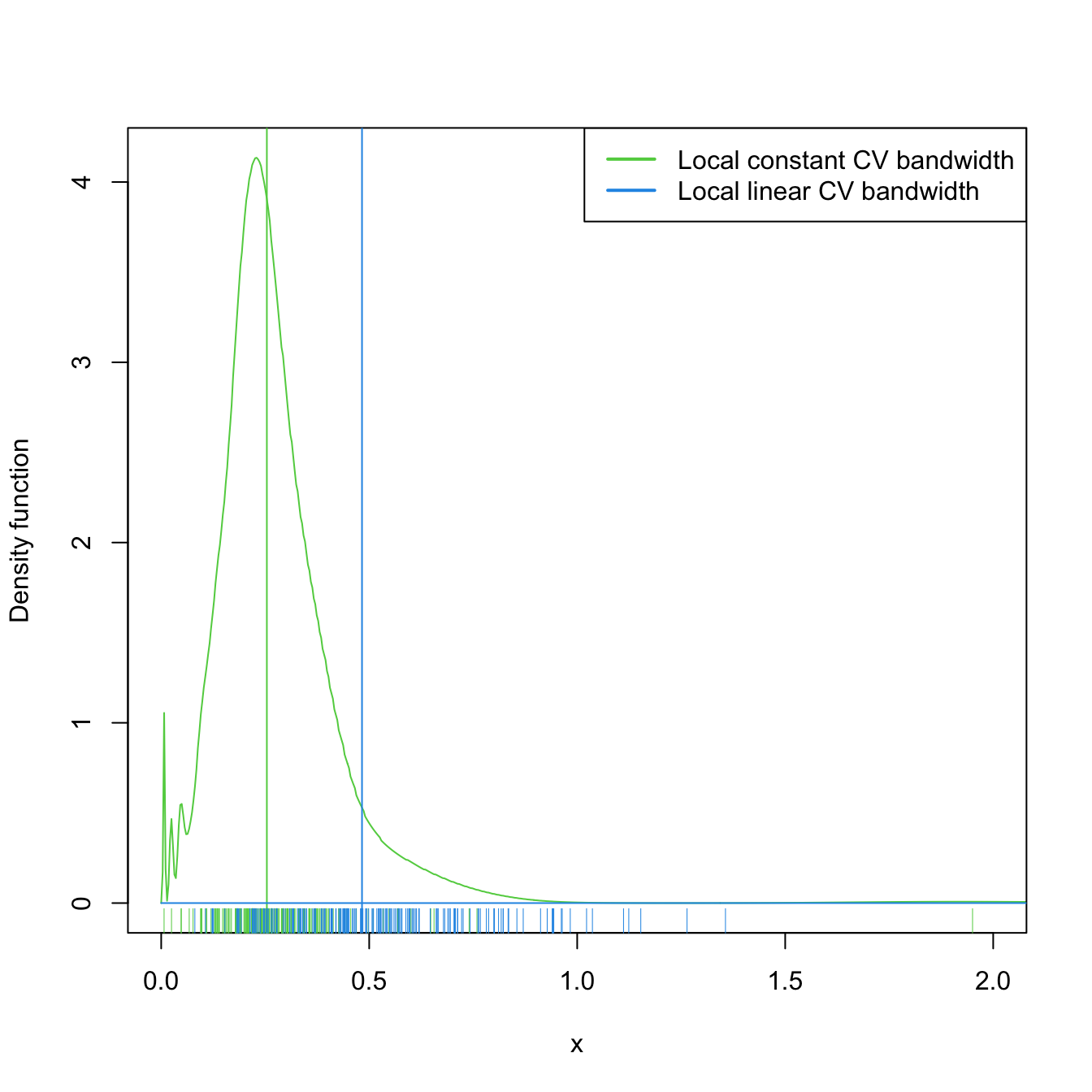
Figure 4.5: Estimated density for the local constant and local linear CV bandwidths, for the setting described in Exercise 4.18. The vertical bars denote the median CV bandwidths. Observe how local linear bandwidths tend to be larger than local constant ones.

Exercise 4.19 Perform the following simulation study for each of the local constant and local linear estimators.

Plot the regression function $m(x)=x\cos(x).$
Simulate $n=100$ observations from the regression model $Y=m(X)+\varepsilon,$ where $\frac{1}{2}X$ is distributed according to a nor1mix::MW.nm7 and $\varepsilon\sim\mathcal{N}(0, 1).$
Compute the CV bandwidths and the fit associated with this bandwidth.
Plot the fit as a line. Trick: adjust the transparency of each line for better visualization.
Repeat Steps 2–4 $M=75$ times.

The two outputs should be similar to Figure 4.6.

$Local constant and linear estimators of the regression function in the setting described in Exercise 4.19. The support of the predictor $X$ has a “hole”, which makes both estimators to behave erratically at that region. The local linear estimator, driven by a local linear fit, may deviate stronger from $m$ than the local constant.$ $Local constant and linear estimators of the regression function in the setting described in Exercise 4.19. The support of the predictor $X$ has a “hole”, which makes both estimators to behave erratically at that region. The local linear estimator, driven by a local linear fit, may deviate stronger from $m$ than the local constant.$

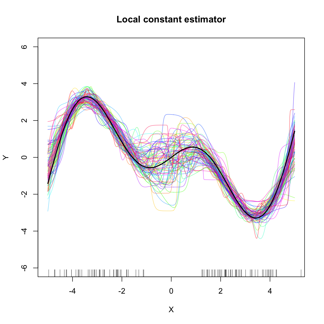
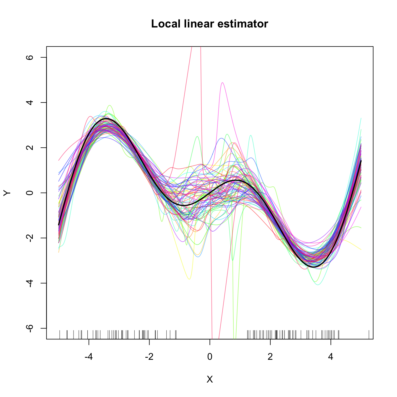
Figure 4.6: Local constant and linear estimators of the regression function in the setting described in Exercise 4.19. The support of the predictor $X$ has a “hole”, which makes both estimators to behave erratically at that region. The local linear estimator, driven by a local linear fit, may deviate stronger from $m$ than the local constant.

There are more sophisticated options for bandwidth selection available in np::npregbw. For example, the argument bwtype allows estimating data-driven variable bandwidths $\hat{h}(x)$ that depend on the evaluation point $x,$ rather than fixed bandwidths $\hat{h},$ as we have considered so far. Roughly speaking, these variable bandwidths are related to the variable bandwidth $\hat{h}_k(x)$ that is necessary to contain the $k$ nearest neighbors $X_1,\ldots,X_k$ of $x$ in the neighborhood $(x-\hat{h}_k(x),x+\hat{h}_k(x)).$ There is an interesting potential gain in employing variable bandwidths, as the local polynomial estimator can adapt the amount of smoothing according to the density of the predictor, therefore avoiding the aforementioned problems related to “holes” in the support of $X$ (see the code below). The extra flexibility of variable bandwidths change the asymptotic properties of the local polynomial estimator. We do not investigate this approach in detail¹⁶¹ but rather point out to its implementation via np.

# Generate some data with bimodal density
set.seed(12345)
n <- 100
eps <- rnorm(2 * n, sd = 2)
m <- function(x) x^2 * sin(x)
X <- c(rnorm(n, mean = -2, sd = 0.5), rnorm(n, mean = 2, sd = 0.5))
Y <- m(X) + eps
x_grid <- seq(-10, 10, l = 500)

# Constant bandwidth
bwc <- np::npregbw(formula = Y ~ X, bwtype = "fixed",
                   regtype = "ll")
krec <- np::npreg(bwc, exdat = x_grid)

# Variable bandwidths
bwg <- np::npregbw(formula = Y ~ X, bwtype = "generalized_nn",
                   regtype = "ll")
kreg <- np::npreg(bwg, exdat = x_grid)
bwa <- np::npregbw(formula = Y ~ X, bwtype = "adaptive_nn",
                   regtype = "ll")
krea <- np::npreg(bwa, exdat = x_grid)

# Comparison
plot(X, Y)
rug(X, side = 1); rug(Y, side = 2)
lines(x_grid, m(x_grid), col = 1)
lines(krec$eval$x_grid, krec$mean, col = 2)
lines(kreg$eval$x_grid, kreg$mean, col = 3)
lines(krea$eval$x_grid, krea$mean, col = 4)
legend("top", legend = c("True regression", "Fixed", "Generalized NN",
                         "Adaptive NN"),
       lwd = 2, col = 1:4)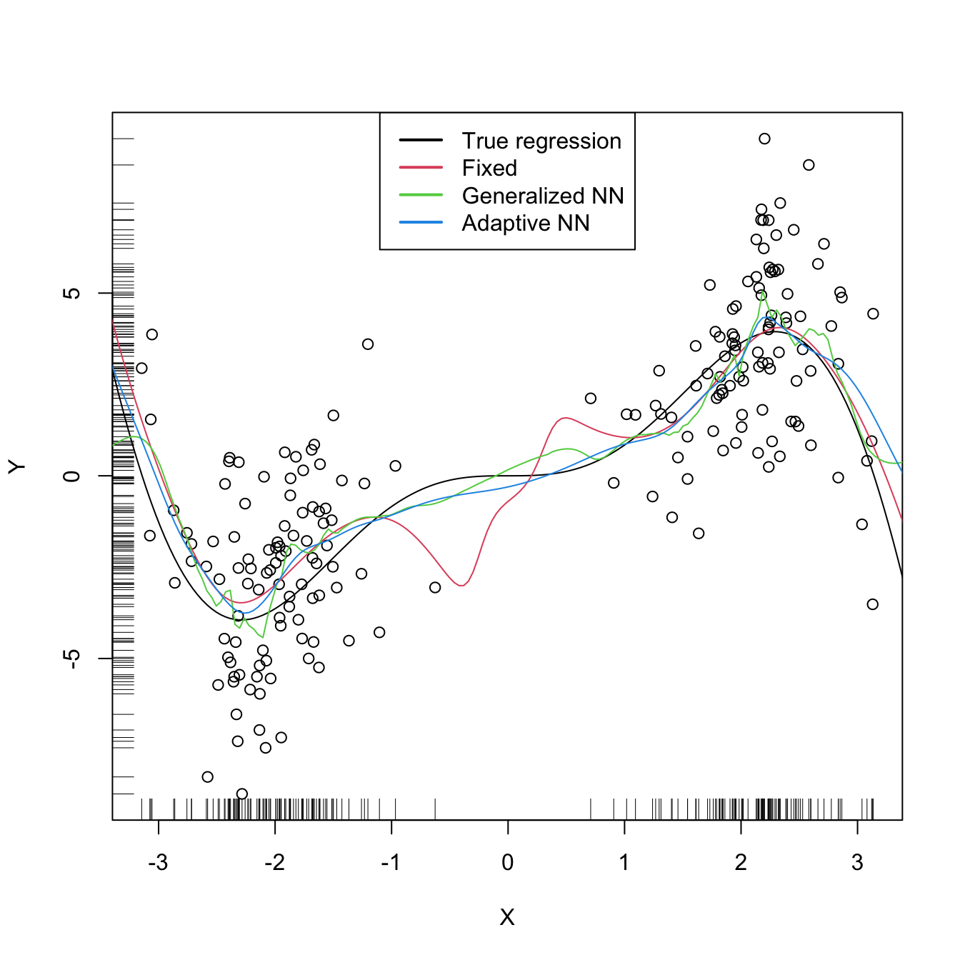

# Observe how the fixed bandwidth may yield a fit that produces serious
# artifacts in the low-density region. At that region the NN-based bandwidths
# expand to borrow strength from the points in the high-density regions,
# whereas in the high-density regions they shrink to adapt faster to the
# changes of the regression function

Exercise 4.20 Repeat Exercise 4.19 replacing Step 3 with:

Compute the variable bandwidths bwtype = "generalized_nn" and bwtype = "adaptive_nn" and the fits associated with them.

Describe the obtained results. Are they qualitatively different from those based on fixed bandwidths, given in Figure 4.6? Do the fits improve with variable bandwidths?

Exercise 4.21 Consider the data(sunspots_births, package = "rotasym") dataset. Then:

Filter the dataset to account only for the 23rd cycle.
Inspect the graphical relation between dist_sun_disc (response) and log10(total_area + 1) (predictor).
Compute the CV bandwidth for the above regression, for the local constant estimator.
Compute and plot the local constant estimator using CV bandwidth. Comment on the fit.
Repeat c and d for the local linear estimator.
Are your conclusions in part e the same for the 21st and 22nd cycles?

References

Hayfield, T., and J. S. Racine. 2008. “Nonparametric Econometrics: The np Package.” Journal of Statistical Software 27 (5): 1–32. https://doi.org/10.18637/jss.v027.i05.

Li, Q., and J. S. Racine. 2007. Nonparametric Econometrics. Princeton: Princeton University Press. https://press.princeton.edu/books/hardcover/9780691121611/nonparametric-econometrics.

The interested reader is referred to Chapter 14 in Li and Racine (2007) and references therein.↩︎