2.1 Histograms

2.1.1 Histogram

The simplest method to estimate a density $f$ from an iid sample $X_1,\ldots,X_n$ is the histogram. From an analytical point of view, the idea is to aggregate the data in intervals of the form $[x_0,x_0+h)$ and then use their relative frequency to approximate the density at $x\in[x_0,x_0+h),$ $f(x),$ by the estimate of¹⁵

$$\begin{align*} f(x_0)&=F'(x_0)\\ &=\lim_{h\to0^+}\frac{F(x_0+h)-F(x_0)}{h}\\ &=\lim_{h\to0^+}\frac{\mathbb{P}[x_0<X< x_0+h]}{h}. \end{align*}$$

More precisely, given an origin $t_0$ and a bandwidth $h>0,$ the histogram builds a piecewise constant function in the intervals $\{B_k:=[t_{k},t_{k+1}):t_k=t_0+hk,k\in\mathbb{Z}\}$ by counting the number of sample points inside each of them. These constant-length intervals are also called bins. The fact that they are of constant length $h$ is important: we can easily standardize the counts on any bin by $h$ in order to have relative frequencies per length¹⁶ in the bins. The histogram at a point $x$ is defined as

$$\begin{align} \hat{f}_\mathrm{H}(x;t_0,h):=\frac{1}{nh}\sum_{i=1}^n1_{\{X_i\in B_k:x\in B_k\}}. \tag{2.1} \end{align}$$

Equivalently, if we denote the number of observations $X_1,\ldots,X_n$ in $B_k$ as $v_k,$ then the histogram can be written as

$$\begin{align*} \hat{f}_\mathrm{H}(x;t_0,h)=\frac{v_k}{nh},\quad\text{ if }x\in B_k\text{ for a certain }k\in\mathbb{Z}. \end{align*}$$

The computation of histograms is straightforward in R. As an example, we consider the old-but-gold faithful dataset. This dataset contains the duration of the eruption and the waiting time between eruptions for the Old Faithful geyser in Yellowstone National Park (USA).

# The faithful dataset is included in R
head(faithful)
##   eruptions waiting
## 1     3.600      79
## 2     1.800      54
## 3     3.333      74
## 4     2.283      62
## 5     4.533      85
## 6     2.883      55

# Duration of eruption
faith_eruptions <- faithful$eruptions

# Default histogram: automatically chosen bins and absolute frequencies!
histo <- hist(faith_eruptions)

# List that contains several objects
str(histo)
## List of 6
##  $ breaks  : num [1:9] 1.5 2 2.5 3 3.5 4 4.5 5 5.5
##  $ counts  : int [1:8] 55 37 5 9 34 75 54 3
##  $ density : num [1:8] 0.4044 0.2721 0.0368 0.0662 0.25 ...
##  $ mids    : num [1:8] 1.75 2.25 2.75 3.25 3.75 4.25 4.75 5.25
##  $ xname   : chr "faith_eruptions"
##  $ equidist: logi TRUE
##  - attr(*, "class")= chr "histogram"

# With relative frequencies
hist(faith_eruptions, probability = TRUE)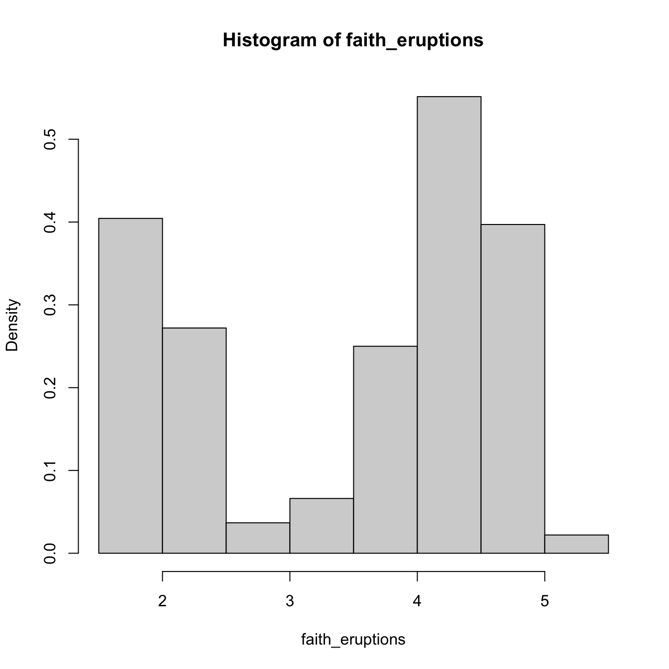

# Choosing the breaks
# t0 = min(faithE), h = 0.25
Bk <- seq(min(faith_eruptions), max(faith_eruptions), by = 0.25)
hist(faith_eruptions, probability = TRUE, breaks = Bk)
rug(faith_eruptions) # Plotting the sample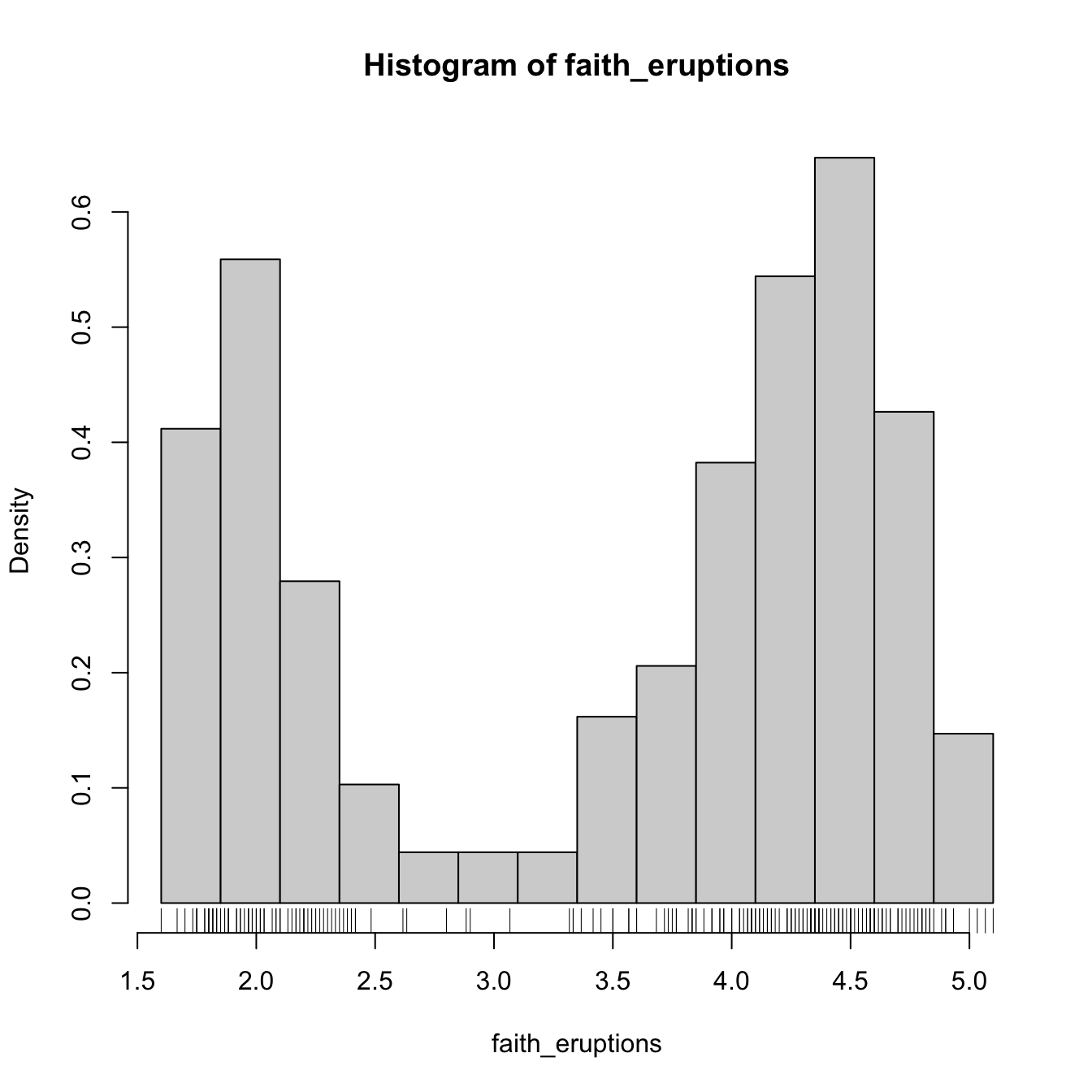

Exercise 2.1 For iris$Sepal.Length, compute:

1. The histogram of relative frequencies with five bins.
2. The histogram of absolute frequencies with $t_0=4.3$ and $h=1.$

Add the rug of the data for both histograms.

The analysis of $\hat{f}_\mathrm{H}(x;t_0,h)$ as a random variable is simple, once one recognizes that the bin counts $v_k$ are distributed as $\mathrm{B}(n,p_k),$ with $p_k:=\mathbb{P}[X\in B_k]=\int_{B_k} f(t)\,\mathrm{d}t.$¹⁷ If $f$ is continuous, then by the integral mean value theorem, $p_k=hf(\xi_{k,h})$ for a $\xi_{k,h}\in(t_k,t_{k+1}).$ Assume that $k\in\mathbb{Z}$ is such that $x\in B_k=\lbrack t_k,t_{k+1}).$¹⁸ Therefore:

$$\begin{align} \begin{split} \mathbb{E}[\hat{f}_\mathrm{H}(x;t_0,h)]&=\frac{np_k}{nh}=f(\xi_{k,h}),\\ \mathbb{V}\mathrm{ar}[\hat{f}_\mathrm{H}(x;t_0,h)]&=\frac{np_k(1-p_k)}{n^2h^2}=\frac{f(\xi_{k,h})(1-hf(\xi_{k,h}))}{nh}. \end{split} \tag{2.2} \end{align}$$

The results above yield interesting insights:

1. If $h\to0,$ then $\xi_{k,h}\to x,$¹⁹ resulting in $f(\xi_{k,h})\to f(x),$ and thus (2.1) becomes an asymptotically (when $h\to0$) unbiased estimator of $f(x).$
2. But if $h\to0,$ the variance increases. For decreasing the variance, $nh\to\infty$ is required.
3. The variance is directly dependent on $f(\xi_{k,h})(1-hf(\xi_{k,h}))\to f(x)$ (as $h\to0$), hence there is more variability at regions with higher density.

A more detailed analysis of the histogram can be seen in Section 3.2.2 in Scott (2015). We skip it since the detailed asymptotic analysis for the more general kernel density estimator will be given in Section 2.2.

Exercise 2.2 Given (2.2), obtain $\mathrm{MSE}[\hat{f}_\mathrm{H}(x;t_0,h)].$ What should happen in order to have $\mathrm{MSE}[\hat{f}_\mathrm{H}(x;t_0,h)]\to0$?

Clearly, the shape of the histogram depends on:

• $t_0,$ since the separation between bins happens at $t_0+kh,$ $k\in\mathbb{Z};$
• $h,$ which controls the bin size and the effective number of bins for aggregating the sample.

We focus first on exploring the dependence on $t_0,$ as it serves for motivating the next density estimator.

# Sample from a U(0, 1)
set.seed(1234567)
u <- runif(n = 100)

# Bins for t0 = 0, h = 0.2
Bk1 <- seq(0, 1, by = 0.2)

# Bins for t0 = -0.1, h = 0.2
Bk2 <- seq(-0.1, 1.1, by = 0.2)

# Comparison of histograms for different t0's
hist(u, probability = TRUE, breaks = Bk1, ylim = c(0, 1.5),
     main = "t0 = 0, h = 0.2")
rug(u)
abline(h = 1, col = 2)
hist(u, probability = TRUE, breaks = Bk2, ylim = c(0, 1.5),
     main = "t0 = -0.1, h = 0.2")
rug(u)
abline(h = 1, col = 2)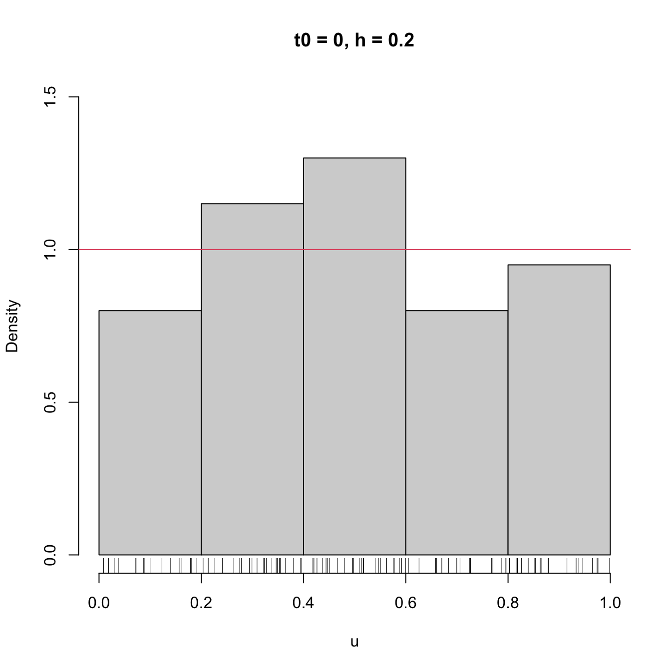

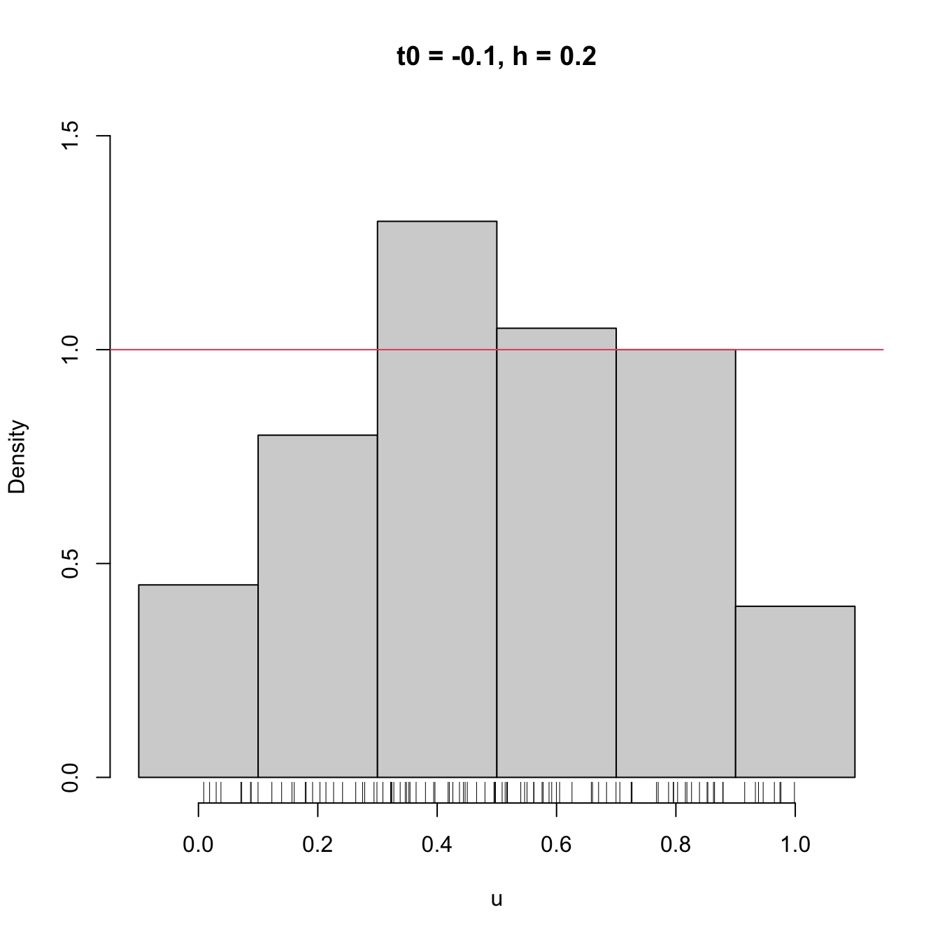
Figure 2.2: The dependence of the histogram on the origin $t_0.$ The red curve represents the uniform pdf.

High dependence on $t_0$ also happens when estimating densities that are not compactly supported. The following snippet of code points towards it.

# Sample 50 points from a N(0, 1) and 25 from a N(3.25, 0.25)
set.seed(1234567)
samp <- c(rnorm(n = 50, mean = 0, sd = 1),
          rnorm(n = 25, mean = 3.25, sd = sqrt(0.5)))

# min and max for choosing Bk1 and Bk2
range(samp)
## [1] -2.082486  4.344547

# Comparison
Bk1 <- seq(-2.5, 5, by = 0.5)
Bk2 <- seq(-2.25, 5.25, by = 0.5)
hist(samp, probability = TRUE, breaks = Bk1, ylim = c(0, 0.5),
     main = "t0 = -2.5, h = 0.5")
curve(2/3 * dnorm(x, mean = 0, sd = 1) +
        1/3 * dnorm(x, mean = 3.25, sd = sqrt(0.5)), col = 2, add = TRUE,
      n = 200)
rug(samp)
hist(samp, probability = TRUE, breaks = Bk2, ylim = c(0, 0.5),
     main = "t0 = -2.25, h = 0.5")
curve(2/3 * dnorm(x, mean = 0, sd = 1) +
        1/3 * dnorm(x, mean = 3.25, sd = sqrt(0.5)), col = 2, add = TRUE,
      n = 200)
rug(samp)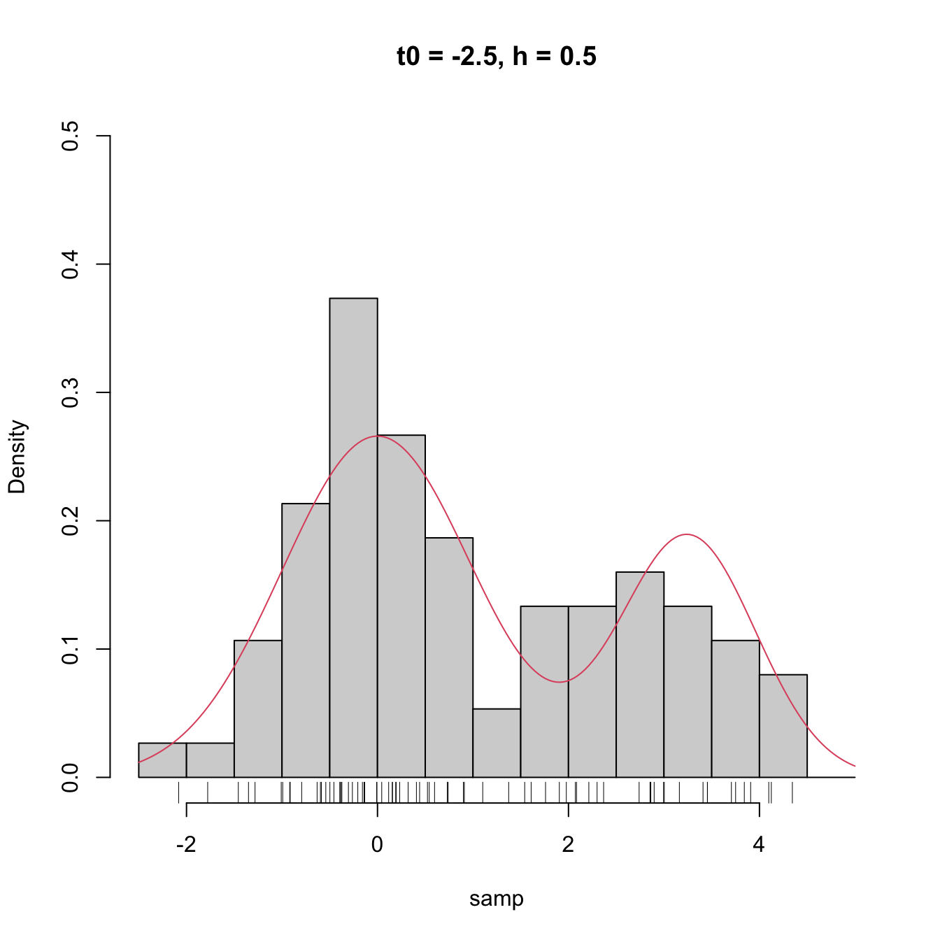

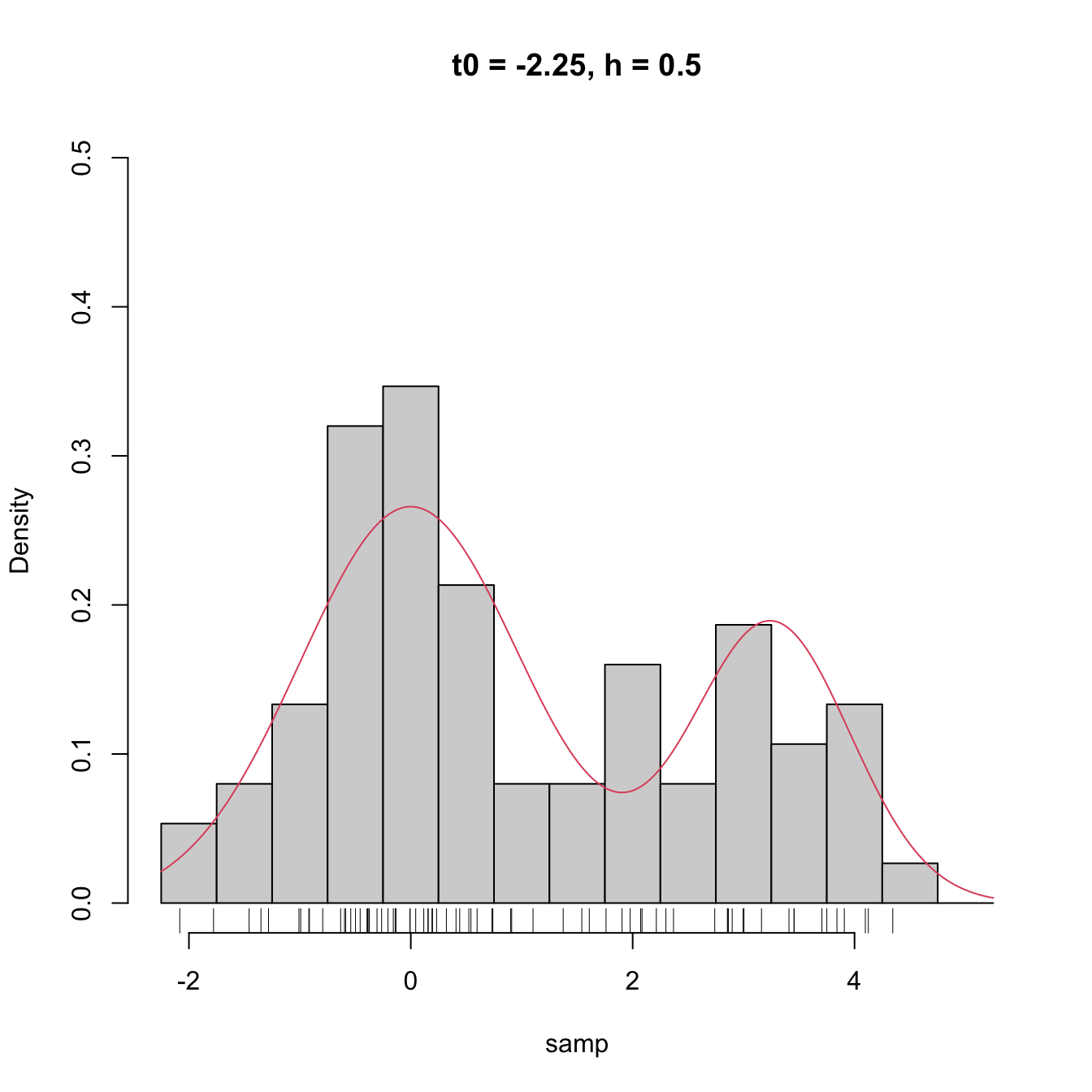
Figure 2.3: The dependence of the histogram on the origin $t_0$ for non-compactly supported densities. The red curve represents the underlying pdf, a mixture of two normals.

Clearly, the subjectivity introduced by the dependence of $t_0$ is something that we would like to get rid of. We can do so by allowing the bins to be dependent on $x$ (the point at which we want to estimate $f(x)$), rather than fixing them beforehand.

2.1.2 Moving histogram

An alternative to avoid the dependence on $t_0$ is the moving histogram, also known as the naive density estimator.²⁰ The idea is to aggregate the sample $X_1,\ldots,X_n$ in intervals of the form $(x-h, x+h)$ and then use its relative frequency in $(x-h,x+h)$ to approximate the density at $x,$ which can be expressed as

$$\begin{align*} f(x)&=F'(x)\\ &=\lim_{h\to0^+}\frac{F(x+h)-F(x-h)}{2h}\\ &=\lim_{h\to0^+}\frac{\mathbb{P}[x-h<X<x+h]}{2h}. \end{align*}$$

Recall the differences with the histogram: the intervals depend on the evaluation point $x$ and are centered about it. This allows us to directly estimate $f(x)$ (without the proxy $f(x_0)$) using an estimate based on the symmetric derivative of $F$ at $x,$ instead of employing an estimate based on the forward derivative of $F$ at $x_0.$

More precisely, given a bandwidth $h>0,$ the naive density estimator builds a piecewise constant function by considering the relative frequency of $X_1,\ldots,X_n$ inside $(x-h,x+h)$:

$$\begin{align} \hat{f}_\mathrm{N}(x;h):=\frac{1}{2nh}\sum_{i=1}^n1_{\{x-h<X_i<x+h\}}. \tag{2.3} \end{align}$$

Figure 2.4 shows the moving histogram for the same sample used in Figure 2.3, clearly revealing the remarkable improvement with respect to the histograms shown when estimating the underlying density.

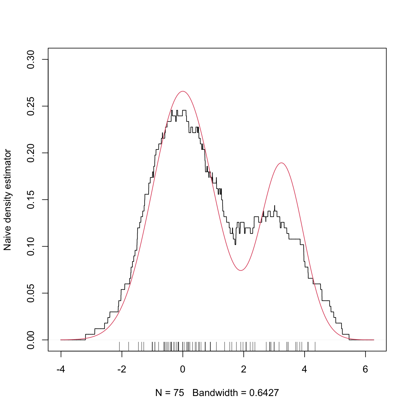
Figure 2.4: The naive density estimator $\hat{f}_\mathrm{N}(\cdot;h)$ (black curve). The red curve represents the underlying pdf, a mixture of two normals.

Exercise 2.3 Is $\hat{f}_\mathrm{N}(\cdot;h)$ continuous in general? Justify your answer. If the answer is negative, then:

1. What is the maximum number of discontinuities it may have?
2. What should happen to have fewer discontinuities than its maximum?

Exercise 2.4 Implement your own version of the moving histogram in R. It must be a function that takes as inputs:

1. a vector with the evaluation points $x;$
2. sample $X_1,\ldots,X_n;$
3. bandwidth $h.$

The function must return (2.3) evaluated for each $x.$ Test the implementation by comparing the density of a $\mathcal{N}(0, 1)$ when estimated with $n=100$ observations.

Analogously to the histogram, the analysis of $\hat{f}_\mathrm{N}(x;h)$ as a random variable follows from realizing that

$$\begin{align*} &\sum_{i=1}^n1_{\{x-h<X_i<x+h\}}\sim \mathrm{B}(n,p_{x,h}),\\ &p_{x,h}:=\mathbb{P}[x-h<X<x+h]=F(x+h)-F(x-h). \end{align*}$$

Then:

$$\begin{align} \mathbb{E}[\hat{f}_\mathrm{N}(x;h)]=&\,\frac{F(x+h)-F(x-h)}{2h},\tag{2.4}\\ \mathbb{V}\mathrm{ar}[\hat{f}_\mathrm{N}(x;h)]=&\,\frac{F(x+h)-F(x-h)}{4nh^2}\nonumber\\ &-\frac{(F(x+h)-F(x-h))^2}{4nh^2}.\tag{2.5} \end{align}$$

Exercise 2.5 Derive expressions (2.4) and (2.5) from the binomial relation indicated above.

Results (2.4) and (2.5) provide interesting insights into the effect of $h$:

1. If $h\to0,$ then:

   • $\mathbb{E}[\hat{f}_\mathrm{N}(x;h)]\to f(x)$ and (2.3) is an asymptotically unbiased estimator of $f(x).$
   • $\mathbb{V}\mathrm{ar}[\hat{f}_\mathrm{N}(x;h)]\approx \frac{f(x)}{2nh}-\frac{f(x)^2}{n}\to\infty.$

2. If $h\to\infty,$ then:

   • $\mathbb{E}[\hat{f}_\mathrm{N}(x;h)]\to 0.$
   • $\mathbb{V}\mathrm{ar}[\hat{f}_\mathrm{N}(x;h)]\to0.$

3. The variance shrinks to zero if $nh\to\infty.$²¹ So both the bias and the variance can be reduced if $n\to\infty,$ $h\to0,$ and $nh\to\infty,$ simultaneously.

4. The variance is almost proportional²² to $f(x).$

The animation in Figure 2.5 illustrates the previous points and gives insights into how the performance of (2.3) varies smoothly with $h.$

Figure 2.5: Bias and variance for the moving histogram. The animation shows how for small bandwidths the bias of $\hat{f}_\mathrm{N}(x;h)$ on estimating $f(x)$ is small, but the variance is high, and how for large bandwidths the bias is large and the variance is small. The variance is visualized through the asymptotic $95\%$ confidence intervals for $\hat{f}_\mathrm{N}(x;h).$ Application available here.

The estimator (2.3) raises an important question:

Why give the same weight to all $X_1,\ldots,X_n$ in $(x-h, x+h)$ for approximating $\frac{\mathbb{P}[x-h<X<x+h]}{2h}$?

We are estimating $f(x)=F'(x)$ by estimating $\frac{F(x+h)-F(x-h)}{2h}$ through the relative frequency of $X_1,\ldots,X_n$ in the interval $(x-h,x+h).$ Therefore, it seems reasonable that the data points closer to $x$ are more important to assess the infinitesimal probability of $x$ than the ones further away. This observation shows that (2.3) is indeed a particular case of a wider and more sensible class of density estimators, which we will see next.

References

Scott, D. W. 2015. Multivariate Density Estimation. Second. Wiley Series in Probability and Statistics. Hoboken: John Wiley & Sons. https://doi.org/10.1002/9781118575574.

---

15. Note that we estimate $f(x)$ by means of an estimate for $f(x_0),$ where $x$ is at most $h>0$ units above $x_0.$ Thus, we do not estimate directly $f(x)$ with the histogram.↩︎

16. Recall that, with this standardization, we approach to the probability density concept.↩︎

17. Note that it is key that the $\{B_k\}$ are deterministic (and not sample-dependent) for this result to hold.↩︎

18. This is an important point. Notice also that this $k$ depends on $h$ because $t_k=t_0+kh,$ therefore the $k$ for which $x\in\lbrack t_k,t_{k+1})$ will change when, for example, $h\to0.$↩︎

19. Because $x\in \lbrack t_k,t_{k+1})$ with $k$ changing as $h\to0$ (see the previous footnote) and the interval ends up collapsing in $x,$ so any point in $\lbrack t_k,t_{k+1})$ converges to $x.$↩︎

20. The motivation for this terminology will be apparent in Section 2.2.↩︎

21. Or, in other words, if $h^{-1}=o(n),$ i.e., if $h^{-1}$ grows more slowly than $n$ does.↩︎

22. Why so?↩︎