6.3 Independence tests

Assume that a bivariate iid sample $(X_1,Y_1),\ldots,(X_n,Y_n)$ from an arbitrary distribution $F_{X,Y}$ is given. We next address the independence problem of testing the existence of possible dependence between $X$ and $Y.$

Differently to the previous sections, we will approach this problem through the use of coefficients that capture, up to different extension, the degree of dependence between $X$ and $Y.$²⁶⁴ $\!\!^,$²⁶⁵

6.3.1 Concordance-based tests

Concordance measures

The random variables $X$ and $Y$ are concordant if “large” values of one tend to be associated with “large” values of the other and, analogously, “small” values of one with “small” values of the other. More precisely, given $(x_i,y_i)$ and $(x_j,y_j),$ two observations of $(X,Y),$ we say that:

• $(x_i,y_i)$ and $(x_j,y_j)$ are concordant if $x_i<x_j$ and $y_i<y_j,$ or if $x_i>x_j$ and $y_i>y_j.$
• $(x_i,y_i)$ and $(x_j,y_j)$ are discordant if $x_i>x_j$ and $y_i<y_j,$ or if $x_i<x_j$ and $y_i>y_j.$

Alternatively, $(x_i,y_i)$ and $(x_j,y_j)$ are concordant/discordant depending on whether $(x_i-x_j)(y_i-y_j)$ is positive or negative. Therefore, the concordance concept is similar to the correlation concept, but with a main foundational difference: the former does not use the value of $(x_i-x_j)(y_i-y_j),$ only its sign. Consequently, whether $X$ and $Y$ are concordant or discordant will not be driven by its linear association, as happens with positive/negative correlation. One can think about concordance/discordance as a generalized form of positive/negative correlation.

We say that $X$ and $Y$ are concordant/discordant if the “majority” of the observations of $(X,Y)$ are concordant/discordant. This “majority” is quantified by a certain concordance measure. Many concordance measures exist, with different properties and interpretations. Scarsini (1984) gave an axiomatic definition of the properties that any valid concordance measure for continuous random variables must satisfy.

Definition 6.1 (Concordance measure) A measure $\kappa$ of dependence between two continuous random variables $X$ and $Y$ is a concordance measure if it satisfies the following axioms:

1. Domain: $\kappa(X,Y)$ is defined for any $(X,Y)$ with continuous cdf.
2. Symmetry: $\kappa(X,Y)=\kappa(Y,X).$
3. Coherence: $\kappa(X,Y)$ is monotone in $C_{X,Y}$ (the copula of $(X,Y)$).²⁶⁶ That is, if $C_{X,Y}\geq C_{W,Z},$ then $\kappa(X,Y)\geq \kappa(W,Z).$²⁶⁷
4. Range: $-1\leq\kappa(X,Y)\leq1.$
5. Independence: $\kappa(X,Y)=0$ if $X$ and $Y$ are independent.
6. Change of sign: $\kappa(-X,Y)=-\kappa(X,Y).$
7. Continuity: if $(X,Y)\sim H$ and $(X_n,Y_n)\sim H_n,$ and if $H_n$ converges pointwise to $H$ (and $H_n$ and $H$ continuous), then $\lim_{n\to\infty} \kappa(X_n,Y_n)=\kappa(X,Y).$²⁶⁸

The next theorem, less technical, gives direct insight into what a concordance measure brings on top of correlation: characterize if $(X,Y)$ is such that one variable can be “perfectly predicted” from the other.²⁶⁹ Perfect prediction can only be achieved if each continuous variable is a monotone function $g$ of the other.²⁷⁰

Theorem 6.1 Let $\kappa$ be a concordance measure for two continuous random variables $X$ and $Y$:

1. If $Y=g(X)$ (almost surely) and $g$ is an increasing function, then $\kappa(X,Y)=1.$
2. If $Y=g(X)$ (almost surely) and $g$ is a decreasing function, then $\kappa(X,Y)=-1.$
3. If $\alpha$ and $\beta$ are strictly monotonic functions almost everywhere in the supports of $X$ and $Y,$ then $\kappa(\alpha(X),\beta(Y))=\kappa(X,Y).$

Remark. Correlation is not a concordance measure. For example, it fails to verify the third property of Theorem 6.1: $\mathrm{Cor}[X,Y]= \mathrm{Cor}[\alpha(X),\beta(Y)]$ is true only if $\alpha$ and $\beta$ are linear functions.

Important for our interests is Axiom v: independence implies a zero concordance measure, for any proper concordance measure. Note that the converse is false. However, since dependence often manifests itself in concordance patterns, testing independence by testing zero concordance is a useful approach with a more informative rejection of $H_0.$

Kendall’s tau and Spearman’s rho

The two most famous measures of concordance for $(X,Y)$ are Kendall’s tau and Spearman’s rho. Both can be regarded as generalizations of $\mathrm{Cor}[X,Y]$ that are not driven by linear relations; rather, they look into the concordance of $(X,Y)$ and the monotone relation between $X$ and $Y.$

The Kendall’s tau of $(X,Y),$ denoted by $\tau(X,Y),$ is defined as

$$\begin{align} \tau(X,Y):=&\,\mathbb{P}[(X-X')(Y-Y')>0]\nonumber\\ &-\mathbb{P}[(X-X')(Y-Y')<0],\tag{6.29} \end{align}$$

where $(X',Y')$ is an iid copy of $(X,Y).$²⁷¹ $\!\!^,$²⁷² That is, $\tau(X,Y)$ is the difference of the concordance and discordance probabilities between two random observations of $(X,Y).$

The Spearman’s rho of $(X,Y),$ denoted by $\rho(X,Y),$ is defined as

$$\begin{align} \rho(X,Y):=&\,3\big\{\mathbb{P}[(X-X')(Y-Y'')>0]\nonumber\\ &-\mathbb{P}[(X-X')(Y-Y'')<0]\big\},\tag{6.30} \end{align}$$

where $(X',Y')$ and $(X'',Y'')$ are two iid copies from $(X,Y).$²⁷³ Recall that $(X',Y'')$ is a random vector that, by construction, has independent components with marginals equal to those of $(X,Y).$ Hence, $(X',Y'')$ is the “independence version” of $(X,Y)$.²⁷⁴ Therefore, $\rho(X,Y)$ is proportional to the difference of the concordance and discordance probabilities between two random observations, one from $(X,Y)$ and another from its independence version.

A neater interpretation of the Spearman’s rho follows from the following other equivalent definition:

$$\begin{align} \rho(X,Y)=\mathrm{Cor}[F_X(X),F_Y(Y)],\tag{6.31} \end{align}$$

where $F_X$ and $F_Y$ are the marginal cdfs of $X$ and $Y,$ respectively. Expression (6.31) hides the concordance view of $\rho(X,Y),$ but it states that the Spearman’s rho between two random variables is the correlation between their probability transforms.²⁷⁵

Exercise 6.21 Obtain (6.31) from (6.30). Hint: prove first the equality for $X\sim\mathcal{U}(0,1)$ and $Y\sim\mathcal{U}(0,1).$

Although different, Kendall’s tau and Spearman’s rho are heavily related. For example, it is impossible to have $\tau(X,Y)=-0.5$ and $\rho(X,Y)=0.5$ for the same continuous random vector $(X,Y).$ Their relation can be precisely visualized in Figure 6.11, which shows the feasibility region for $(\tau,\rho)$ given by Theorem 6.2. The region is the optimal possible and cannot be narrowed.

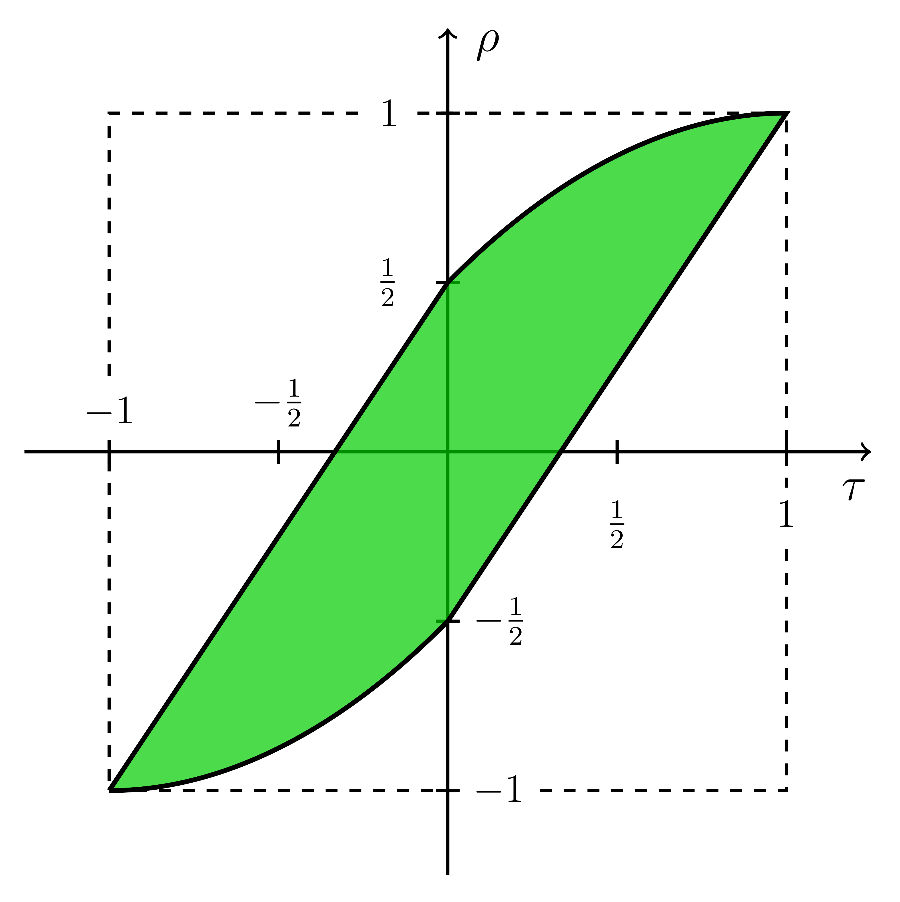
Figure 6.11: Feasible region for $(\tau,\rho)$ given by Theorem 6.2.

Theorem 6.2 Let $X$ and $Y$ be two continuous random variables with $\tau\equiv\tau(X,Y)$ and $\rho\equiv\rho(X,Y).$ Then,

$$\begin{align*} \frac{3\tau-1}{2}\leq &\;\rho\leq\frac{1+2\tau-\tau^2}{2},&&\tau\geq 0,\\ \frac{\tau^2+2\tau-1}{2}\leq &\;\rho\leq\frac{1+3\tau}{2},&&\tau\leq 0. \end{align*}$$

Kendall’s tau and Spearman’s rho tests of no concordance

• Tests purpose. Given $(X_1,Y_1),\ldots,(X_n,Y_n)\sim F_{X,Y},$ test $H_0:\tau=0$ vs. $H_1:\tau\neq0,$ and $H_0:\rho=0$ vs. $H_1:\rho\neq0.$²⁷⁶

• Statistics definition. The tests are based on the sample versions of (6.29) and (6.31):

  $$\begin{align} \hat\tau:=&\,\frac{c-d}{\binom{n}{2}}=\frac{2(c-d)}{n(n-1)},\tag{6.32}\\ \hat\rho:=&\,\frac{\sum_{i=1}^n(R_i-\bar{R})(S_i-\bar{S})}{\sqrt{\sum_{i=1}^n(R_{i}-\bar{R})^2 \sum_{i=1}^n(S_{i}-\bar{S})^2}},\tag{6.33} \end{align}$$

  where $c=\sum_{\substack{i,j=1\\i<j}}^n 1_{\{(X_i-X_j)(Y_i-Y_j)>0\}}$ denotes the number of concordant pairs in the sample, $d=\binom{n}{2}-c$ is the number of discordant pairs, and $R_i:=\mathrm{rank}_X(X_i)=nF_{X,n}(X_i)$ and $S_i:=\mathrm{rank}_Y(Y_i)=nF_{Y,n}(Y_i),$ $i=1,\ldots,n$ are the ranks of the samples of $X$ and $Y.$

  Large positive (negative) values of $\hat\tau$ and $\hat\rho$ indicate presence of concordance (discordance) between $X$ and $Y.$ The two-sided tests reject $H_0$ for large absolute values of $\hat\tau$ and $\hat\rho.$

• Statistics computation. Formulae (6.32) and (6.33) are reasonably explicit, but the latter can be improved to

  $$\begin{align*} \hat\rho=1-\frac{6}{n(n^2-1)}\sum_{i=1}^n(R_i-S_i)^2. \end{align*}$$

  The naive computation of $\hat\tau$ involves $O(n^2)$ operations, hence it escalates to large sample sizes worse than $\hat\rho.$ A faster implementation of $O(n\log(n))$ is available through pcaPP::cor.fk.

• Distributions under $H_0.$ The asymptotic null distributions of $\hat\tau$ and $\hat\rho$ follow from

  $$\begin{align*} \sqrt{\frac{9n(n-1)}{2(2n+5)}}\hat{\tau}\stackrel{d}{\longrightarrow}\mathcal{N}(0,1),\quad \sqrt{n-1}\hat{\rho}\stackrel{d}{\longrightarrow}\mathcal{N}(0,1) \end{align*}$$

  under $H_0.$ Exact distributions are available for small $n$’s.

• Highlights and caveats. Both $\tau=0$ and $\rho=0$ do not characterize independence. Therefore, absence of rejection does not guarantee lack of evidence in favor of dependence. Rejection of $H_0$ does guarantee the existence of significant dependence, in the form of concordance (positive values of $\hat\tau$ and $\hat\rho$) or discordance (negative values). Both tests are distribution-free.

• Implementation in R. The test statistics $\hat\tau$ and $\hat\rho$ and the exact/asymptotic $p$-values are available through the cor.test function, specifying method = "kendall" or method = "spearman". The default alternative = "two.sided" carries out the two-sided tests for $H_1:\tau\neq 0$ and $H_1:\rho\neq 0.$ The one-sided alternatives follows with alternative = "greater" ($>0$) and alternative = "less" ($<0$).

The following chunk of code illustrates the use of cor.test. It also gives some examples of the advantages of $\hat\tau$ and $\hat\rho$ over the correlation coefficient.

# Outliers fool correlation, but do not fool concordance
set.seed(123456)
n <- 200
x <- rlnorm(n)
y <- rlnorm(n)
y[n] <- x[n] <- 5e2
cor.test(x, y, method = "pearson") # Close to 1 due to outlier
## 
##  Pearson's product-moment correlation
## 
## data:  x and y
## t = 189.72, df = 198, p-value < 2.2e-16
## alternative hypothesis: true correlation is not equal to 0
## 95 percent confidence interval:
##  0.9963800 0.9979276
## sample estimates:
##       cor 
## 0.9972609
cor.test(x, y, method = "kendall") # Close to 0, as it should
## 
##  Kendall's rank correlation tau
## 
## data:  x and y
## z = -0.89189, p-value = 0.3725
## alternative hypothesis: true tau is not equal to 0
## sample estimates:
##         tau 
## -0.04241206
cor.test(x, y, method = "spearman") # Close to 0, as it should
## 
##  Spearman's rank correlation rho
## 
## data:  x and y
## S = 1419086, p-value = 0.3651
## alternative hypothesis: true rho is not equal to 0
## sample estimates:
##         rho 
## -0.06434111
cor(rank(x), rank(y)) # Spearman's rho
## [1] -0.06434111
plot(x, y, main = "Massive outlier introduces spurious correlation",
     pch = 16)
abline(lm(y ~ x), col = 2, lwd = 2)

plot(rank(x), rank(y), main = "Concordance is unaffected by outliers",
     pch = 16)
abline(lm(rank(y) ~ rank(x)), col = 2, lwd = 2)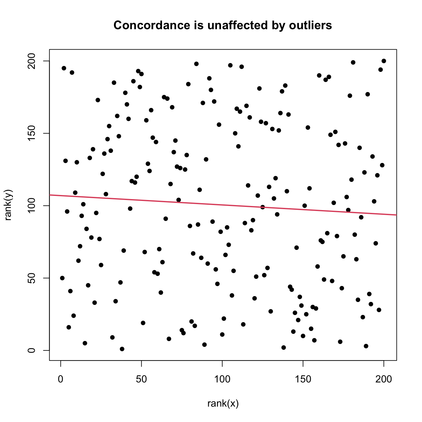

# Outliers fool the sign of correlation, but do not fool concordance
x <- 1000 + rlnorm(n)
y <- x
x[n] <- 1500
y[n] <- 250
cor.test(x, y, method = "pearson", alternative = "greater") # Change of sign!
## 
##  Pearson's product-moment correlation
## 
## data:  x and y
## t = -153.49, df = 198, p-value = 1
## alternative hypothesis: true correlation is greater than 0
## 95 percent confidence interval:
##  -0.9966951  1.0000000
## sample estimates:
##       cor 
## -0.995824
cor.test(x, y, method = "kendall", alternative = "greater") # Fine
## 
##  Kendall's rank correlation tau
## 
## data:  x and y
## z = 20.608, p-value < 2.2e-16
## alternative hypothesis: true tau is greater than 0
## sample estimates:
##  tau 
## 0.98
cor.test(x, y, method = "spearman", alternative = "greater") # Fine
## 
##  Spearman's rank correlation rho
## 
## data:  x and y
## S = 39800, p-value < 2.2e-16
## alternative hypothesis: true rho is greater than 0
## sample estimates:
##       rho 
## 0.9701493
plot(x, y, main = "Massive outlier changes the correlation sign",
     pch = 16)
abline(lm(y ~ x), col = 2, lwd = 2)

plot(rank(x), rank(y), main = "Concordance is unaffected by outliers",
     pch = 16)
abline(lm(rank(y) ~ rank(x)), col = 2, lwd = 2)

However, as previously said, concordance measures do not characterize independence. Below are some dependence situations that are undetected by $\hat\tau$ and $\hat\rho.$

# Non-monotone dependence fools concordance
set.seed(123456)
n <- 200
x <- rnorm(n)
y <- abs(x) + rnorm(n)
cor.test(x, y, method = "kendall")
## 
##  Kendall's rank correlation tau
## 
## data:  x and y
## z = -1.5344, p-value = 0.1249
## alternative hypothesis: true tau is not equal to 0
## sample estimates:
##         tau 
## -0.07296482
cor.test(x, y, method = "spearman")
## 
##  Spearman's rank correlation rho
## 
## data:  x and y
## S = 1473548, p-value = 0.1381
## alternative hypothesis: true rho is not equal to 0
## sample estimates:
##        rho 
## -0.1051886
plot(x, y, main = "Undetected non-monotone dependence", pch = 16)
abline(lm(y ~ x), col = 2)

plot(rank(x), rank(y), main = "Undetected non-monotone dependence in ranks",
     pch = 16)
abline(lm(rank(y) ~ rank(x)), col = 2, lwd = 2)

# Dependence in terms of conditional variance fools concordance
x <- rnorm(n)
y <- rnorm(n, sd = abs(x))
cor.test(x, y, method = "kendall")
## 
##  Kendall's rank correlation tau
## 
## data:  x and y
## z = 1.0271, p-value = 0.3044
## alternative hypothesis: true tau is not equal to 0
## sample estimates:
##        tau 
## 0.04884422
cor.test(x, y, method = "spearman")
## 
##  Spearman's rank correlation rho
## 
## data:  x and y
## S = 1251138, p-value = 0.3857
## alternative hypothesis: true rho is not equal to 0
## sample estimates:
##        rho 
## 0.06162304
plot(x, y, main = "Undetected heteroscedasticity", pch = 16)
abline(lm(y ~ x), col = 2)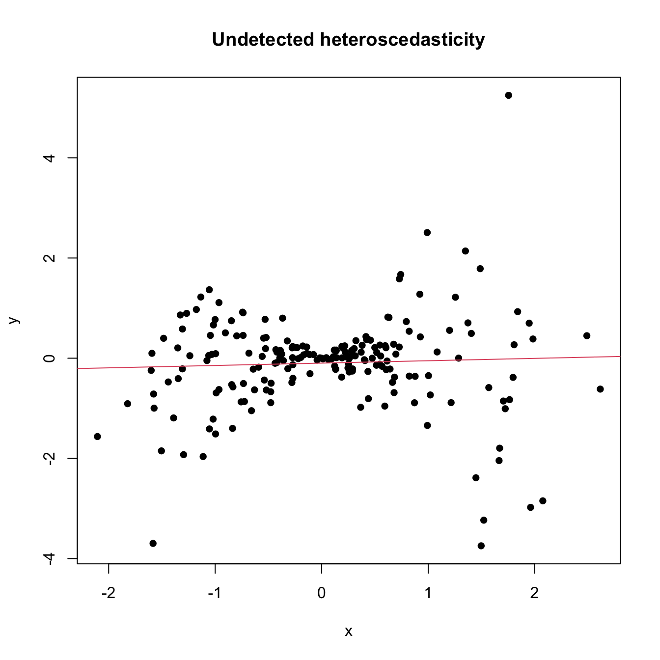

plot(rank(x), rank(y), main = "Undetected heteroscedasticity in ranks",
     pch = 16)
abline(lm(rank(y) ~ rank(x)), col = 2, lwd = 2)

6.3.2 Distance correlation tests

A characterization of independence

No-concordance tests based on $\hat\tau$ and $\hat\rho$ are easy to interpret and carry out, but they are not omnibus for testing independence: they do not detect all kinds of dependence between $X$ and $Y,$ only those expressible with $\tau\neq0$ and $\rho\neq0.$ Therefore, and as evidenced previously, Kendall’s tau and Spearman’s rho may not detect dependence patterns in the form of non-monotone relations or heteroscedasticity.

The handicap of concordance measures on not being able to detect all kinds of dependence has been recently solved by Székely, Rizzo, and Bakirov (2007) with the introduction of a new type of correlation measure that completely characterizes independence.²⁷⁷ This new type of correlation is not a correlation between values of $(X,Y).$ Rather, it is related to the correlation between pairwise distances of $X$ and $Y.$ The following definitions, adapted from Section 7.1 in Székely and Rizzo (2017), give the precise form of distance covariance and distance variance between two random variables $X$ and $Y,$ which are the pillars of a distance correlation.

Definition 6.2 (Distance covariance and variance) The distance covariance (dCov) between two random variables $X$ and $Y$ with $\mathbb{E}[|X|]<\infty$ and $\mathbb{E}[|Y|]<\infty$ is the nonnegative number $\mathcal{V}(X,Y)$ with square equal to

$$\begin{align} \mathcal{V}^2(X, Y):=&\,\mathbb{E}\left[|X-X'||Y-Y'|\right]+\mathbb{E}\left[|X-X'|\right] \mathbb{E}\left[|Y-Y'|\right] \nonumber\\ &-2 \mathbb{E}\left[|X-X'||Y-Y''|\right] \tag{6.34}\\ =&\,\mathrm{Cov}\left[|X-X'|,|Y-Y'|\right] \nonumber\\ &- 2\mathrm{Cov}\left[|X-X'|,|Y-Y''|\right],\tag{6.35} \end{align}$$

where $(X',Y')$ and $(X'',Y'')$ are iid copies of $(X,Y).$ The distance variance (dVar) of $X$ is defined as

$$\begin{align} \mathcal{V}^2(X):=&\,\mathcal{V}^2(X, X) \nonumber\\ =&\,\mathbb{V}\mathrm{ar}\left[|X-X'|\right] - 2\mathrm{Cov}\left[|X-X'|,|X-X''|\right].\tag{6.36} \end{align}$$

Some interesting points implicit in Definition 6.2 are:

• dCov is unsigned: dCov does not inform on the “direction” of the dependence between $X$ and $Y.$

• From (6.34), it is clear that $\mathcal{V}(X, Y)=0$ if $X$ and $Y$ are independent, as in that case $\mathbb{E}\left[|X-X'||Y-Y'|\right] = \mathbb{E}\left[|X-X'|\right]\mathbb{E}\left[|Y-Y'|\right] = \mathbb{E}\left[|X-X'||Y-Y''|\right].$

• Equation (6.34) is somehow reminiscent of Spearman’s rho (see (6.30)) and uses $(X',Y''),$ the independence version of $(X,Y).$

• As (6.35) points out, dCov is not the covariance between pairwise distances of $X$ and $Y,$ $\mathrm{Cov}\left[|X-X'|,|Y-Y'|\right].$ However, $\mathcal{V}^2(X, Y)$ is related to such covariances: it can be regarded as a covariance between pairwise distances that is “centered” by the covariances of the “independent versions” of the pairwise distances:

  $$\begin{align*} \mathcal{V}^2(X, Y)=&\,\mathrm{Cov}\left[|X-X'|,|Y-Y'|\right]\\ &- \mathrm{Cov}\left[|X-X'|,|Y-Y''|\right]- \mathrm{Cov}\left[|X-X''|,|Y-Y'|\right]. \end{align*}$$

Distance correlation is defined analogously to how correlation is defined from covariance and variance.

Definition 6.3 (Distance correlation) The distance correlation (dCor) between two random variables $X$ and $Y$ with $\mathbb{E}[|X|]<\infty$ and $\mathbb{E}[|Y|]<\infty$ is the nonnegative number $\mathcal{R}(X, Y)$ with square equal to

$$\begin{align} \mathcal{R}^2(X, Y):=\frac{\mathcal{V}^2(X, Y)}{\sqrt{\mathcal{V}^2(X) \mathcal{V}^2(Y)}}\tag{6.37} \end{align}$$

if $\mathcal{V}^2(X) \mathcal{V}^2(Y)>0.$ If $\mathcal{V}^2(X) \mathcal{V}^2(Y)=0,$ then $\mathcal{R}^2(X, Y):=0.$

The following theorem collects useful properties of dCov, dVar, and dCor. Some of them are related to the properties of standard covariance (recall, e.g., (1.3)) and (unsigned) correlation. However, as anticipated, Property iv gives the clear edge of dCor over concordance measures on completely characterizing independence.

Theorem 6.3 (Properties of dCov, dVar, and dCor) Let $X$ and $Y$ be two random variables with $\mathbb{E}[|X|]<\infty$ and $\mathbb{E}[|Y|]<\infty.$ Then:

1. $\mathcal{V}(a+bX, c+dY)=\sqrt{|bd|}\mathcal{V}(X, Y)$ for all $a,b,c,d\in\mathbb{R}.$
2. $\mathcal{V}(a+bX)=|b|\mathcal{V}(X)$ for all $a,b\in\mathbb{R}.$
3. If $\mathcal{V}(X)=0,$ then $X=\mathbb{E}[X]$ almost surely.
4. $\mathcal{R}(X,Y)=\mathcal{V}(X,Y)=0$ if and only if $X$ and $Y$ are independent.
5. $0\leq \mathcal{R}(X,Y)\leq 1.$
6. If $\mathcal{R}(X,Y) = 1,$ then there exist $a,b\in\mathbb{R},$ $b\neq0,$ such that $Y = a + bX.$
7. If $(X,Y)$ is normally distributed and is such that $\mathrm{Cor}[X,Y]=\rho,$ $-1\leq\rho\leq 1,$ then $$\begin{align*} \mathcal{R}^2(X, Y)=\frac{\rho \sin^{-1}(\rho)+\sqrt{1-\rho^2}-\rho \sin^{-1}(\rho/2)-\sqrt{4-\rho^2}+1}{1+\pi / 3-\sqrt{3}} \end{align*}$$ and $\mathcal{R}(X, Y)\leq |\rho|.$

Figure 6.12: Mapping $\rho\mapsto\mathcal{R}(X(\rho), Y(\rho))$ (in black) for the normally distributed vector $(X(\rho),Y(\rho))$ such that $\mathrm{Cor}\lbrack X(\rho),Y(\rho)\rbrack=\rho.$ In red, the absolute value function $\rho\mapsto|\rho|.$

Two important simplifications have been done on the previous definitions and theorem for the sake of a simplified exposition. Precisely, dCov admits a more general definition that addresses two generalizations, the first one being especially relevant for practical purposes:

1. Multivariate extensions. dCov, dVar, and dCor can be straightforwardly extended to account for multivariate vectors $\mathbf{X}$ and $\mathbf{Y}$ supported on $\mathbb{R}^p$ and $\mathbb{R}^q.$ It is as simple as replacing the absolute values $|\cdot|$ in Definition 6.2 with the Euclidean norms $\|\cdot\|_p$ and $\|\cdot\|_q$ for $\mathbb{R}^p$ and $\mathbb{R}^q,$ respectively. The properties stated in Theorem 6.3 hold once suitably adapted. For example, for $\mathbf{X}$ and $\mathbf{Y}$ such that $\mathbb{E}[\|\mathbf{X}\|_p]<\infty$ and $\mathbb{E}[\|\mathbf{Y}\|_q]<\infty,$ dCov is defined as the square root of $$\begin{align*} \mathcal{V}^2(\mathbf{X}, \mathbf{Y}):=&\,\mathrm{Cov}\left[\|\mathbf{X}-\mathbf{X}'\|_p,\|\mathbf{Y}-\mathbf{Y}'\|_q\right]\\ &- 2\mathrm{Cov}\left[\|\mathbf{X}-\mathbf{X}'\|_p,\|\mathbf{Y}-\mathbf{Y}''\|_q\right] \end{align*}$$ and dVar as $\mathcal{V}^2(\mathbf{X})=\mathcal{V}^2(\mathbf{X}, \mathbf{X}).$ Recall that both dCov and dVar are scalars, whereas $\mathbb{V}\mathrm{ar}[\mathbf{X}]$ is a $p\times p$ matrix. Consequently, the dCor of $\mathbf{X}$ and $\mathbf{Y}$ is also a scalar that condenses all the dependencies between $\mathbf{X}$ and $\mathbf{Y}.$²⁷⁸

2. Characteristic-function view of dCov. dCov does not require $\mathbb{E}[|X|]<\infty$ and $\mathbb{E}[|Y|]<\infty$ to be defined. It can be defined, without resorting to expectations, through the characteristic functions²⁷⁹ of $X,$ $Y,$ and $(X,Y)$: $$\begin{align*} \psi_X(s):=\mathbb{E}[e^{\mathrm{i}sX}],\;\, \psi_Y(t):=\mathbb{E}[e^{\mathrm{i}tY}],\;\, \psi_{X,Y}(s,t):=\mathbb{E}[e^{\mathrm{i}(sX+tY)}], \end{align*}$$ where $s,t\in\mathbb{R}.$ Indeed, $$\begin{align} \mathcal{V}^2(X,Y)=\frac{1}{c_1^2} \int_{\mathbb{R}^2} \big|\psi_{X,Y}(s, t)-\psi_{X}(s) \psi_{Y}(t)\big|^2\frac{\mathrm{d}t \,\mathrm{d}s}{|t|^2|s|^2},\tag{6.38} \end{align}$$ where $c_p:=\pi^{(p+1)/2}/\Gamma((p+1)/2)$ and $|\cdot|$ represents the modulus of a complex number. The alternative definition (6.38) shows that $\mathcal{V}^2(X,Y)$ can be regarded as a weighted squared distance between the joint and marginal characteristic functions, and offers deeper insight into why $\mathcal{V}^2(X,Y)=0$ characterizes independence.²⁸⁰ This alternative view also holds for the multivariate case, where (6.38) becomes²⁸¹ $$\begin{align*} \mathcal{V}^2(\mathbf{X},\mathbf{Y})=\frac{1}{c_pc_q} \int_{\mathbb{R}^p}\int_{\mathbb{R}^q} \big|\psi_{\mathbf{X},\mathbf{Y}}(\mathbf{s}, \mathbf{t})-\psi_{\mathbf{X}}(\mathbf{s}) \psi_{\mathbf{Y}}(\mathbf{t})\big|^2\frac{\mathrm{d}\mathbf{t} \,\mathrm{d}\mathbf{s}}{\|\mathbf{t}\|_q^{q+1}\|\mathbf{s}\|_p^{p+1}}. \end{align*}$$

Distance correlation test

Independence tests for $(X,Y)$ can be constructed by evaluating if $\mathcal{R}(X,Y)$ or $\mathcal{V}(X,Y)=0$ holds. To do so, we first need to consider the empirical versions of dCov and dCor. These follow from (6.34) and (6.37).

Definition 6.4 (Empirical distance covariance and variance) The dCov for the random sample $(X_1,Y_1),\ldots,(X_n,Y_n)$ is the nonnegative number $\mathcal{V}_n(X,Y)$ with square equal to

$$\begin{align} \mathcal{V}_n^2(X,Y):=&\,\frac{1}{n^2} \sum_{k, \ell=1}^n A_{k \ell} B_{k \ell},\tag{6.39} \end{align}$$

where

$$\begin{align*} A_{k \ell}:=&\,a_{k \ell}-\bar{a}_{k \bullet}-\bar{a}_{\bullet \ell}+\bar{a}_{\bullet\bullet},\quad a_{k \ell}:=|X_k-X_\ell|,\\ \bar{a}_{k \bullet}:=&\,\frac{1}{n} \sum_{l=1}^n a_{k \ell},\quad \bar{a}_{\bullet \ell}:=\frac{1}{n} \sum_{k=1}^n a_{k \ell},\quad \bar{a}_{\bullet \bullet}:=\frac{1}{n^2} \sum_{k, \ell=1}^n a_{k \ell}, \end{align*}$$

and $B_{k \ell}:=b_{k \ell}-\bar{b}_{k \bullet}-\bar{b}_{\bullet \ell}+\bar{b}_{\bullet\bullet}$ is defined analogously for $b_{k \ell}:=|Y_k-Y_\ell|.$ The dVar of $X_1,\ldots,X_n$ is defined as $\mathcal{V}_n^2(X):=\frac{1}{n^2} \sum_{k, \ell=1}^n A_{k \ell}^2.$

Definition 6.5 (Empirical distance correlation) The dCor for the random sample $(X_1,Y_1),\ldots,(X_n,Y_n)$ is the nonnegative number $\mathcal{R}_n(X, Y)$ with square equal to

$$\begin{align} \mathcal{R}_n^2(X, Y):=\frac{\mathcal{V}_n^2(X, Y)}{\sqrt{\mathcal{V}_n^2(X) \mathcal{V}_n^2(Y)}}\tag{6.40} \end{align}$$

if $\mathcal{V}_n^2(X) \mathcal{V}_n^2(Y)>0.$ If $\mathcal{V}_n^2(X) \mathcal{V}_n^2(Y)=0,$ then $\mathcal{R}_n^2(X, Y):=0.$

Remark. The previous empirical versions of dCov, dVar, and dCor also allow for multivariate versions. These are based on $a_{k \ell}:=\|\mathbf{X}_k-\mathbf{X}_\ell\|_p$ and $b_{k \ell}:=\|\mathbf{Y}_k-\mathbf{Y}_\ell\|_q.$

We next introduce the independence tests based on (6.39)–(6.40).

• Test purpose. Given $(X_1,Y_1),\ldots,(X_n,Y_n)\sim F_{X,Y},$ test $H_0:F_{X,Y}=F_XF_Y$ vs. $H_1:F_{X,Y}\neq F_XF_Y$ consistently against all the alternatives in $H_1.$

• Statistic definition. The dCov test rejects $H_0$ for large values of the test statistic $n\mathcal{V}_n^2(X,Y)$ (not the dCov!), which indicates a departure from independence. The dCor test uses as test statistic $\mathcal{R}_n^2(X,Y)$ and rejects $H_0$ for large values of it.

• Statistic computation. Formulae (6.39) and (6.40) are directly implementable, yet they involve $O(n^2)$ computations.²⁸²

• Distribution under $H_0.$ If $H_0$ holds, then the asymptotic cdf of $n\mathcal{V}_n^2(X,Y)$ is the cdf of the random variable

  $$\begin{align} \sum_{j=1}^\infty\lambda_j Y_j,\quad \text{where } Y_j\sim\chi^2_1,\,j\geq 1,\text{ are iid}\tag{6.41} \end{align}$$

  and $\{\lambda_j\}_{j=1}^\infty$ are certain nonnegative constants that depend on $F_{X,Y}$ (so the test is not distribution-free). As with (6.8), the cdf of (6.41) does not admit a simple analytical expression. In addition, it is mostly unusable in practice, since $\{\lambda_j\}_{j=1}^\infty$ are unknown. The asymptotic distribution for $\mathcal{R}_n^2(X,Y)$ is related to that of $n\mathcal{V}_n^2(X,Y).$ However, both test statistics can be calibrated by permutations (see Section 6.3.3).

• Highlights and caveats. On the positive side, the dCov/dCor test is much more general than concordance-based tests: (i) it is an omnibus test for independence; and (ii) it can be applied to multivariate data. On the negative side, the dCov/dCor test is not distribution-free, so fast asymptotic $p$-values are not available. Besides, the rejection of the dCov/dCor tests does not inform on the kind of dependence between $X$ and $Y.$ The dCov and dCor tests perform similarly and their computational burdens are roughly equivalent. The dCor test offers the edge of having an absolute scale for its test statistic, since $\mathcal{R}_n^2(X,Y)\in[0,1].$

• Implementation in R. The energy package implements both tests through the energy::dcov.test and energy::dcor.test functions, which compute the test statistics and give $p$-values approximated by permutations (see Section 6.3.3).

The use of energy::dcov.test and energy::dcor.test for testing the independence between $X$ and $Y$ is shown in the following chunk of code.

# Distance correlation detects non-monotone dependence
set.seed(123456)
n <- 200
x <- rnorm(n)
y <- abs(x) + rnorm(n)

# Distance covariance and correlation tests. R is the number of permutations
# and needs to be specified (the default is R = 0 -- no test is produced)
energy::dcov.test(x, y, R = 1e3)
## 
##  dCov independence test (permutation test)
## 
## data:  index 1, replicates 1000
## nV^2 = 6.4595, p-value = 0.001998
## sample estimates:
##      dCov 
## 0.1797145
energy::dcor.test(x, y, R = 1e3)
## 
##  dCor independence test (permutation test)
## 
## data:  index 1, replicates 1000
## dCor = 0.26188, p-value = 0.000999
## sample estimates:
##      dCov      dCor   dVar(X)   dVar(Y) 
## 0.1797145 0.2618840 0.6396844 0.7361771

# Distance correlation detects conditional variance as dependence
x <- rnorm(n)
y <- rnorm(n, sd = abs(x))

# Distance covariance and correlation tests
energy::dcov.test(x, y, R = 1e3)
## 
##  dCov independence test (permutation test)
## 
## data:  index 1, replicates 1000
## nV^2 = 3.5607, p-value = 0.001998
## sample estimates:
##      dCov 
## 0.1334296
energy::dcor.test(x, y, R = 1e3)
## 
##  dCor independence test (permutation test)
## 
## data:  index 1, replicates 1000
## dCor = 0.25031, p-value = 0.004995
## sample estimates:
##      dCov      dCor   dVar(X)   dVar(Y) 
## 0.1334296 0.2503077 0.6152985 0.4618172

Testing the independence of two random vectors $\mathbf{X}$ and $\mathbf{Y}$ is also straightforward, as the code below illustrates.

# A multivariate case with independence
set.seed(123456)
n <- 200
p <- 5
x <- matrix(rnorm(n * p), nrow = n, ncol = p)
y <- matrix(rnorm(n * p), nrow = n, ncol = p)
energy::dcov.test(x, y, R = 1e3)
## 
##  dCov independence test (permutation test)
## 
## data:  index 1, replicates 1000
## nV^2 = 8.5627, p-value = 0.7493
## sample estimates:
##      dCov 
## 0.2069139
energy::dcor.test(x, y, R = 1e3)
## 
##  dCor independence test (permutation test)
## 
## data:  index 1, replicates 1000
## dCor = 0.28323, p-value = 0.7732
## sample estimates:
##      dCov      dCor   dVar(X)   dVar(Y) 
## 0.2069139 0.2832256 0.7163536 0.7450528

# A multivariate case with dependence
y <- matrix(0.2 * rnorm(n = n * p, mean = c(x)) +
              rnorm(n * p, sd = 1.25), nrow = n, ncol = p)
energy::dcov.test(x, y, R = 1e3)
## 
##  dCov independence test (permutation test)
## 
## data:  index 1, replicates 1000
## nV^2 = 14.592, p-value = 0.01099
## sample estimates:
##      dCov 
## 0.2701076
energy::dcor.test(x, y, R = 1e3)
## 
##  dCor independence test (permutation test)
## 
## data:  index 1, replicates 1000
## dCor = 0.32299, p-value = 0.007992
## sample estimates:
##      dCov      dCor   dVar(X)   dVar(Y) 
## 0.2701076 0.3229851 0.7163536 0.9762951

Exercise 6.22 Illustrate with a simulation study the performance of the independence tests for $(X,Y)$ based on Pearson’s correlation, Spearman’s rho, and distance covariance. To that end, use five simulation scenarios and build a $5\times 4$ plot such that:

• The first column contains illustrative scatterplots of the generated data.
• The second, third, and fourth column show histograms of the $p$-values of Pearson’s correlation, Spearman’s rho, and distance covariance tests in that scenario, respectively.

For the four scenarios, consider: (1) independence; (2) an alternative where Pearson’s correlation test has the largest power; (3) an alternative where Spearman’s rho has the largest power; (4) an alternative for which all tests have similar powers; (5) an undetectable alternative by Spearman’s rho. Choose the scenarios originally and in such a way the histograms of the $p$-values are not completely extreme. Use $M=1,000$ Monte Carlo replicates and set $n=100.$ Use permutations to obtain the $p$-values in all tests for a fairer comparison, setting $B=500.$ Explain the obtained results.

6.3.3 Permutation-based approach to testing independence

The calibration of a test of independence can be approached by permutations, in an analogous way as that carried out in Section 6.2.3 for tests of homogeneity. None of the permutation strategies previously seen is adequate, though, since the independence problem, expressed as

$$\begin{align*} H_0:F_{X,Y}=F_XF_Y\quad\text{vs.}\quad H_1:F_{X,Y}\neq F_XF_Y, \end{align*}$$

is substantially different from (6.13). Here, $F_{X,Y}$ represents the joint cdf of $(X,Y),$ $F_X$ and $F_Y$ stand for the corresponding marginal cdfs, and “$F_{X,Y}\neq F_XF_Y$” denotes that there exists at least one $(x,y)\in\mathbb{R}^2$ such that $F_{X,Y}(x,y)\neq F_X(x)F_Y(y).$

In the unpaired homogeneity case, the elements of the samples $X_1,\ldots,X_n$ and $Y_1,\ldots,Y_m$ are randomly exchanged using the pooled sample. In the paired case, the components of each pair $(X_1,Y_1),\ldots,(X_n,Y_n)$ are randomly exchanged. When testing for independence, each of the two sample components of $(X_1,Y_1),\ldots,(X_n,Y_n)$ are separately and randomly exchanged. That the resampling is conducted separately for each component is a direct consequence of the null hypothesis of independence.

Precisely, for any two $n$-permutations $\sigma_1$ and $\sigma_2,$ under independence, it happens that

$$\begin{align*} T_n((X_{\sigma_1(1)},Y_{\sigma_2(1)}),\ldots,(X_{\sigma_1(n)},Y_{\sigma_2(n)}))\stackrel{d}{=}T_n((X_1,Y_1),\ldots,(X_n,Y_n)) \end{align*}$$

for any proper independence test statistic $T_n.$ Furthermore, it is reasonably evident that

$$\begin{align*} T_n((X_{\sigma_1(1)},Y_{\sigma_2(1)}),\ldots,(X_{\sigma_1(n)},Y_{\sigma_2(n)}))=T_n((X_1,Y_{\sigma_3(1)}),\ldots,(X_n,Y_{\sigma_3(n)})) \end{align*}$$

for $\sigma_3(i):=\sigma_2(\sigma_1^{-1}(i)),$ $i\in\{1,\ldots,n\}.$²⁸³ That is, any “double permutation” amounts to “single permutation” and it suffices to permute the second component of the sample (leaving the first component fixed) to attain any of the possible values of $T_n((X_{\sigma_1(1)},Y_{\sigma_2(1)}),\ldots,(X_{\sigma_1(n)},Y_{\sigma_2(n)})).$ From the previous arguments, it follows that

$$\begin{align*} \mathbb{P}[T_n\leq x]=\frac{1}{n!}\sum_{k=1}^{n!} \mathbb{P}[T^{\sigma_k}_n\leq x]\approx \frac{1}{B}\sum_{b=1}^{B} 1_{\big\{T^{\hat{\sigma}_b}_n\leq x\big\}}, \end{align*}$$

where $T^{\sigma}_n\equiv T_n((X_1,Y_{\sigma(1)}),\ldots,(X_n,Y_{\sigma(n)}))$ and $\hat{\sigma}_b,$ $b=1,\ldots,B,$ denote the $B$ randomly-chosen $n$-permutations.

The whole permutation-based procedure for performing an independence test that rejects $H_0$ for large values of the test statistic is summarized below:

1. Compute $T_n\equiv T_n((X_1,Y_1),\ldots,(X_n,Y_n)).$

2. Enter the “permutation world”. For $b=1,\ldots,B$:

   1. Simulate a randomly-permuted sample $Y_1^{*b},\ldots,Y_n^{*b}$ from $\{Y_1,\ldots,Y_n\}.$²⁸⁴
   2. Compute $T_n^{*b}\equiv T_n((X_1,Y_1^{*b}),\ldots,(X_n,Y_n^{*b})).$

3. Obtain the $p$-value approximation

   $$\begin{align*} p\text{-value}\approx\frac{1}{B}\sum_{b=1}^B 1_{\{T_n^{*b}> T_n\}} \end{align*}$$

   and emit a test decision from it. Modify it accordingly if rejection of $H_0$ does not happen for large values of $T_n.$

The following chunk of code provides a template for implementing the previous permutation algorithm.

# A no-association test using the absolute value of Spearman's rho statistic
perm_ind_test <- function(x, B = 1e3, plot_boot = TRUE) {

  # Test statistic function. Requires TWO arguments, one being the original
  # data (X_1, Y_1), ..., (X_n, Y_n) and the other containing the random
  # index for permuting the second component of sample
  Tn <- function(data, perm_index) {

    # Permute sample by perm_index -- only permute the second component
    data[, 2] <- data[, 2][perm_index]

    # Test statistic -- MODIFY DEPENDING ON THE PROBLEM
    abs(cor(x = data[, 1], y = data[, 2], method = "spearman"))

  }

  # Perform permutation resampling with the aid of boot::boot
  Tn_star <- boot::boot(data = x, statistic = Tn, sim = "permutation", R = B)

  # Test information -- MODIFY DEPENDING ON THE PROBLEM
  method <- "Permutation-based Spearman's rho test of no concordance"
  alternative <- "Spearman's rho is not zero"

  # p-value: modify if rejection does not happen for large values of the
  # test statistic. $t0 is the original statistic and $t has the permuted ones.
  pvalue <- mean(Tn_star$t > Tn_star$t0)

  # Construct an "htest" result
  result <- list(statistic = c("stat" = Tn_star$t0), p.value = pvalue,
                 statistic_perm = drop(Tn_star$t),
                 B = B, alternative = alternative, method = method,
                 data.name = deparse(substitute(x)))
  class(result) <- "htest"

  # Plot the position of the original statistic with respect to the
  # permutation replicates?
  if (plot_boot) {

    hist(result$statistic_perm, probability = TRUE,
         main = paste("p-value:", result$p.value),
         xlab = latex2exp::TeX("$T_n^*$"))
    rug(result$statistic_perm)
    abline(v = result$statistic, col = 2, lwd = 2)
    text(x = result$statistic, y = 1.5 * mean(par()$usr[3:4]),
         labels = latex2exp::TeX("$T_n$"), col = 2, pos = 4)

  }

  # Return "htest"
  return(result)

}

# Check the test for H0 true
set.seed(123456)
x0 <- mvtnorm::rmvnorm(n = 100, mean = c(0, 0), sigma = diag(c(1:2)))
ind0 <- perm_ind_test(x = x0, B = 1e3)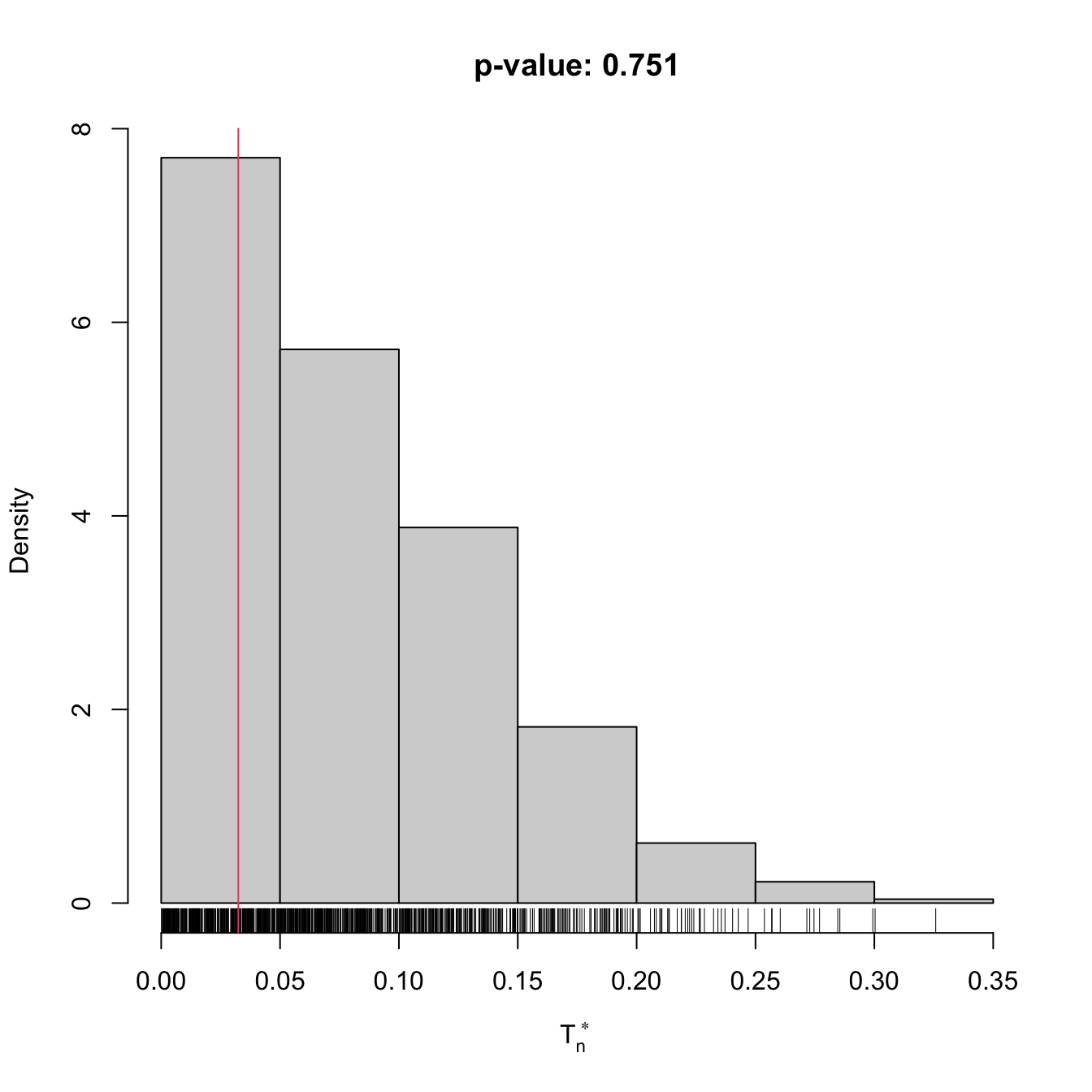

ind0
## 
##  Permutation-based Spearman's rho test of no concordance
## 
## data:  x0
## stat = 0.032439, p-value = 0.751
## alternative hypothesis: Spearman's rho is not zero

# Check the test for H0 false
x1 <- mvtnorm::rmvnorm(n = 100, mean = c(0, 0), sigma = toeplitz(c(1, 0.5)))
ind1 <- perm_ind_test(x = x1, B = 1e3)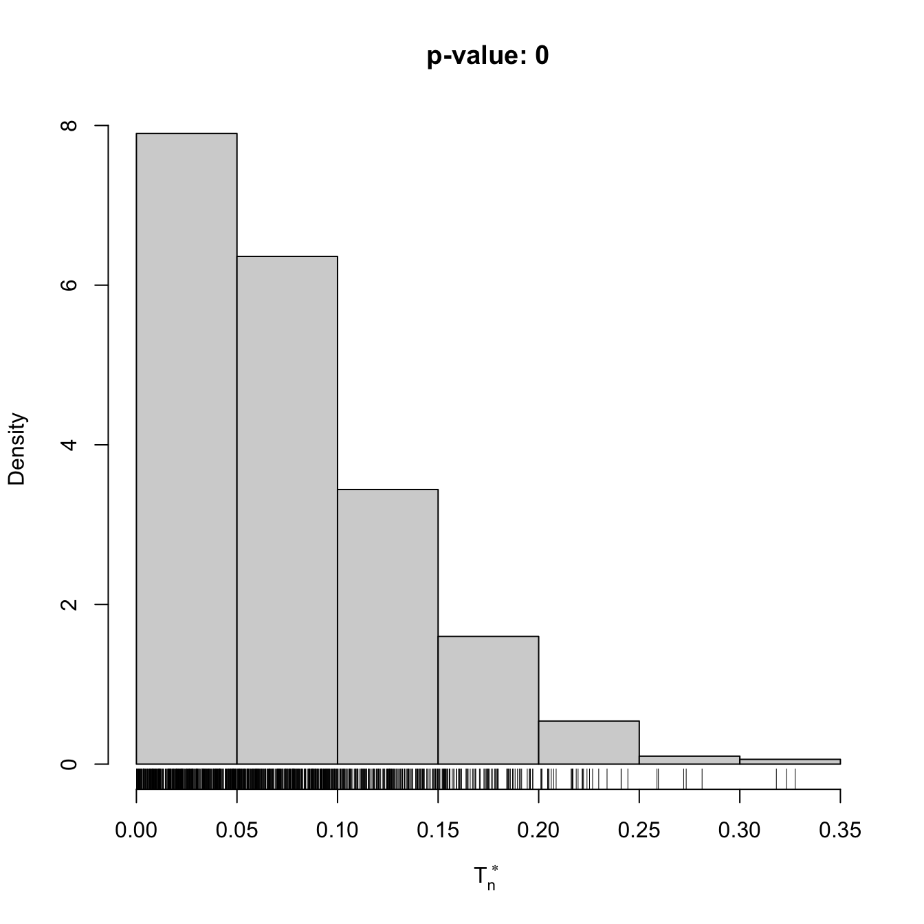

ind1
## 
##  Permutation-based Spearman's rho test of no concordance
## 
## data:  x1
## stat = 0.52798, p-value < 2.2e-16
## alternative hypothesis: Spearman's rho is not zero

References

Blum, J. R., J. Kiefer, and M. Rosenblatt. 1961. “Distribution Free Tests of Independence Based on the Sample Distribution Function.” The Annals of Mathematical Statistics 32 (2): 485–98. https://doi.org/10.1214/aoms/1177705055.

Rizzo, M. L., and G. J. Székely. 2016. “Energy Distance.” WIREs Computational Statistics 8 (1): 27–38. https://doi.org/10.1002/wics.1375.

Scarsini, M. 1984. “On Measures of Concordance.” Stochastica 8: 201–18. https://dmle.icmat.es/revistas/detalle.php?numero=1689.

Székely, G. J., and M. L. Rizzo. 2013. “Energy Statistics: A Class of Statistics Based on Distances.” Journal of Statistical Planning and Inference 143 (8): 1249–72. https://doi.org/10.1016/j.jspi.2013.03.018.

———. 2017. “The Energy of Data.” Annual Review of Statistics and Its Application 4 (1): 447–79. https://doi.org/10.1146/annurev-statistics-060116-054026.

Székely, G. J., M. L. Rizzo, and N. K. Bakirov. 2007. “Measuring and Testing Dependence by Correlation of Distances.” The Annals of Statistics 35 (6): 2769–94. https://doi.org/10.1214/009053607000000505.

---

264. Approaches to independence testing through the ecdf perspective are also possible (see, e.g., Blum, Kiefer, and Rosenblatt (1961)), since the independence of $X$ and $Y$ happens if and only if the joint cdf $F_{X,Y}$ factorizes as $F_XF_Y,$ the product of marginal cdfs. These approaches go along the lines of Sections 6.1.1 and 6.2.↩︎

265. A popular approach to independence and homogeneity testing, not covered in these notes, is the chi-squared test for contingency tables $k\times m$ (see ?chisq.test). This test is applied to a table that contains the observed frequencies of $(X,Y)$ in $km$ classes $I_i\times J_j,$ where $\cup_{i=1}^k I_i$ and $\cup_{j=1}^m J_j$ cover the supports of $X$ and $Y,$ respectively. As with the chi-squared goodness-of-fit test, one can modify the outcome of the test by altering the form of these classes and the choice of $(k,m)$ – a sort of tuning parameter. The choice of $(k,m)$ also affects the quality of the asymptotic null distribution. Therefore, for continuous and discrete random variables, the chi-squared test has significant drawbacks when compared to the ecdf-based tests. However, as opposed to the latter, chi-squared tests can be readily applied to the comparison of categorical variables, where the choice of $(k,m)$ is often more canonical.↩︎

266. The copula $C_{X,Y}$ of a continuous random vector $(X,Y)\sim F_{X,Y}$ is the bivariate function $(u,v)\in[0,1]^2\mapsto C_{X,Y}(u,v)=F_{X,Y}(F_X^{-1}(u),F_Y^{-1}(v))\in[0,1],$ where $F_X$ and $F_Y$ are the marginal cdfs of $X$ and $Y,$ respectively.↩︎

267. That $C_{X,Y}\geq C_{W,Z}$ means that $C_{X,Y}(u,v)\geq C_{W,Z}(u,v)$ for all $(u,v)\in[0,1]^2.$↩︎

268. The assumption is slightly stronger than asking that $(X_n,Y_n)\stackrel{d}{\longrightarrow}(X,Y);$ recall Definition 1.1.↩︎

269. It does not suffice if only $Y$ is perfectly predictable from $X,$ such as in the case $Y=X^2.$↩︎

270. So the function can be inverted almost everywhere, as opposed to the function $g(x)=x^2$ from the previous footnote.↩︎

271. Beware that, here and henceforth, the random variable $X'$ (and not a random vector) is not the transpose of $X.$↩︎

272. $(X',Y')$ is an iid copy of $(X,Y)$ if $(X',Y')\stackrel{d}{=}(X,Y)$ and $(X',Y')$ is independent from $(X,Y).$↩︎

273. An equivalent definition is $\rho(X,Y)=3\big\{\mathbb{P}[(X-X'')(Y-Y')>0]-\mathbb{P}[(X-X'')(Y-Y')<0]\big\}.$↩︎

274. A simple example: if $(X,Y)\sim\mathcal{N}_2(\boldsymbol{\mu},\boldsymbol{\Sigma}),$ then $(X',Y'),(X'',Y'')\sim\mathcal{N}_2(\boldsymbol{\mu},\boldsymbol{\Sigma})$ but $(X',Y'')\sim\mathcal{N}(\mu_1,\sigma_1^2)\times \mathcal{N}(\mu_2,\sigma_2^2).$↩︎

275. Consequently, Spearman’s rho coincides with Pearson’s linear correlation coefficient for uniform variables.↩︎

276. One-sided versions of the tests replace the alternatives by $H_1:\tau>0$ and $H_1:\rho>0,$ or by $H_1:\tau<0$ and $H_1:\rho<0.$↩︎

277. This new type of correlation belongs to a wide class of new statistics that are referred to as energy statistics; see the reviews by Rizzo and Székely (2016) (lighter introduction with R examples), Székely and Rizzo (2013), and Székely and Rizzo (2017) (the latter two being deeper reviews). Energy statistics generate tests alternative to the classical approaches to test goodness-of-fit, normality, homogeneity, independence, and other hypotheses.↩︎

278. In comparison, there are $pq$ (linear) correlations between the entries of $\mathbf{X}$ and $\mathbf{Y}.$↩︎

279. Recall that the characteristic function is a complex-valued function that offers an alternative to the cdf for characterizing the behavior of any random variable.↩︎

280. Two random variables $X$ and $Y$ are independent if and only if $\psi_{X,Y}(s,t)=\psi_{X}(s)\psi_{Y}(t),$ for all $s,t\in\mathbb{R}.$↩︎

281. The characteristic function of a random vector $\mathbf{X}$ is the function $\mathbf{s}\in\mathbb{R}^p\mapsto\psi_{\mathbf{X}}(\mathbf{s}):=\mathbb{E}[e^{\mathrm{i}\mathbf{s}'\mathbf{X}}]\in\mathbb{C}.$↩︎

282. A related bias-corrected estimator of $\mathcal{V}^2(X,Y)$ has been seen to involve $O(n\log n)$ computations (see the discussion in Section 7.2 in Székely and Rizzo (2017)).↩︎

283. Intuitively: once you have the two components permuted, sort the observations in such a way that the first component matches the original sample. Sorting the sample must not affect any proper independence test statistic (we are in the iid case).↩︎

284. This sampling is done by extracting, without replacement, random elements from $\{Y_1,\ldots,Y_n\}.$↩︎