3.1 Multivariate kernel density estimation
Kernel density estimation can be extended to estimate multivariate densities \(f\) in \(\mathbb{R}^p\) based on the same principle: perform an average of densities “centered” at the data points. For a sample \(\mathbf{X}_1,\ldots,\mathbf{X}_n\) in \(\mathbb{R}^p,\) the kde of \(f\) evaluated at \(\mathbf{x}\in\mathbb{R}^p\) is defined as
\[\begin{align} \hat{f}(\mathbf{x};\mathbf{H}):=\frac{1}{n|\mathbf{H}|^{1/2}}\sum_{i=1}^nK\left(\mathbf{H}^{-1/2}(\mathbf{x}-\mathbf{X}_i)\right),\tag{3.1} \end{align}\]
where \(K\) is multivariate kernel, a \(p\)-variate density that is (typically) symmetric and unimodal at \(\mathbf{0},\) and that depends on the bandwidth matrix53 \(\mathbf{H},\) a \(p\times p\) symmetric and positive definite54 matrix.
A common notation is \(K_\mathbf{H}(\mathbf{z}):=|\mathbf{H}|^{-1/2}K\big(\mathbf{H}^{-1/2}\mathbf{z}\big),\) the so-called scaled kernel, so the kde can be compactly written as \(\hat{f}(\mathbf{x};\mathbf{H}):=\frac{1}{n}\sum_{i=1}^nK_\mathbf{H}(\mathbf{x}-\mathbf{X}_i).\) The most employed multivariate kernel is the normal kernel \(K(\mathbf{z})=\phi(\mathbf{z})=(2\pi)^{-p/2}e^{-\frac{1}{2}\mathbf{z}'\mathbf{z}},\) for which \(K_\mathbf{H}(\mathbf{x}-\mathbf{X}_i)=\phi_\mathbf{H}(\mathbf{z}-\mathbf{X}_i).\) Then, the bandwidth \(\mathbf{H}\) can be thought of as the variance-covariance matrix of a multivariate normal density with mean \(\mathbf{X}_i\) and the kde (3.1) can be regarded as a data-driven mixture of those densities.
The interpretation of (3.1) is analogous to the one of (2.7): build a mixture of densities with each density centered at each data point. As a consequence, and roughly speaking, most of the concepts and ideas seen in univariate kernel density estimation extend to the multivariate situation, although some of them have considerable technical complications. For example, bandwidth selection inherits the same cross-validatory ideas (LSCV and BCV selectors) and plug-in methods (NS and DPI) seen before, but with increased complexity for the BCV and DPI selectors.
Exercise 3.1 Using that \(|\mathbf{H}|=\prod_{i=1}^p\lambda_i\) and \(\mathrm{tr}(\mathbf{H})=\sum_{i=1}^p\lambda_i,\) where \(\lambda_1,\ldots,\lambda_p\) are the eigenvalues of \(\mathbf{H},\) find a simple check for a symmetric matrix \(\mathbf{H}\) that guarantees its positive definiteness (and hence its adequacy as a bandwidth for (3.1)) when \(p=2.\)
Recall that considering a full bandwidth matrix \(\mathbf{H}\) gives more flexibility to the kde, but also quadratically increases the amount of bandwidth parameters that need to be chosen – precisely \(\frac{p(p+1)}{2}\) – which notably complicates bandwidth selection as the dimension \(p\) grows, and increases the variance of the kde. A common simplification is to consider a diagonal bandwidth matrix \(\mathbf{H}=\mathrm{diag}(h_1^2,\ldots,h_p^2),\) which yields the kde employing product kernels:
\[\begin{align} \hat{f}(\mathbf{x};\mathbf{h})=\frac{1}{n}\sum_{i=1}^nK_{h_1}(x_1-X_{i,1})\times\stackrel{p}{\cdots}\times K_{h_p}(x_p-X_{i,p}),\tag{3.2} \end{align}\]
where \(\mathbf{X}_i=(X_{i,1},\ldots,X_{i,p})'\) and \(\mathbf{h}=(h_1,\ldots,h_p)'\) is the vector of bandwidths. If the variables \(X_1,\ldots,X_p\) are standardized (so that they have the same scale), then a simple choice is to consider \(h=h_1=\cdots=h_p.\) Diagonal bandwidth matrices will be thoroughly employed when performing kernel regression estimation in Chapter 4.
Multivariate kernel density estimation and bandwidth selection is not supported in base R, but ks::kde implements both for \(p\leq 6.\) In the following code snippet, the functionalities of ks::kde are illustrated for data in \(\mathbb{R}^2.\)
# Simulated data from a bivariate normal
n <- 200
set.seed(35233)
x <- mvtnorm::rmvnorm(n = n, mean = c(0, 0),
                      sigma = rbind(c(1.5, 0.25), c(0.25, 0.5)))

# Compute kde for a diagonal bandwidth matrix (trivially positive definite)
H <- diag(c(1.25, 0.75))
kde <- ks::kde(x = x, H = H)

# The eval.points slot contains the grids on x and y
str(kde$eval.points)
## List of 2
##  $ : num [1:151] -8.58 -8.47 -8.37 -8.26 -8.15 ...
##  $ : num [1:151] -5.1 -5.03 -4.96 -4.89 -4.82 ...

# The grids in kde$eval.points are crossed in order to compute a grid matrix
# where to evaluate the estimate
dim(kde$estimate)
## [1] 151 151

# Manual plotting using the kde object structure
image(kde$eval.points[[1]], kde$eval.points[[2]], kde$estimate,
      col = viridis::viridis(20), xlab = "x", ylab = "y")
points(kde$x) # The data is returned in $x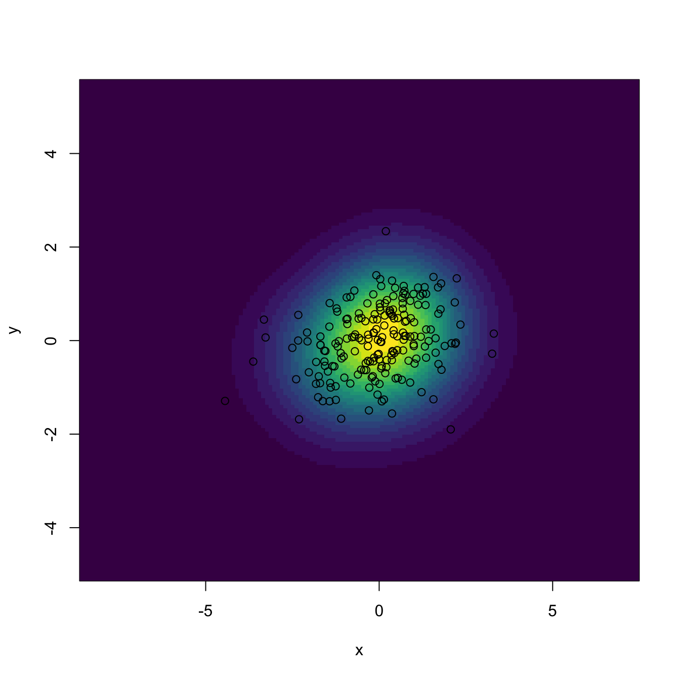
# Changing the grid size to compute the estimates to be 200 x 200 and in the
# rectangle (-4, 4) x c(-3, 3)
kde <- ks::kde(x = x, H = H, gridsize = c(200, 200), xmin = c(-4, -3),
               xmax = c(4, 3))
image(kde$eval.points[[1]], kde$eval.points[[2]], kde$estimate,
      col = viridis::viridis(20), xlab = "x", ylab = "y")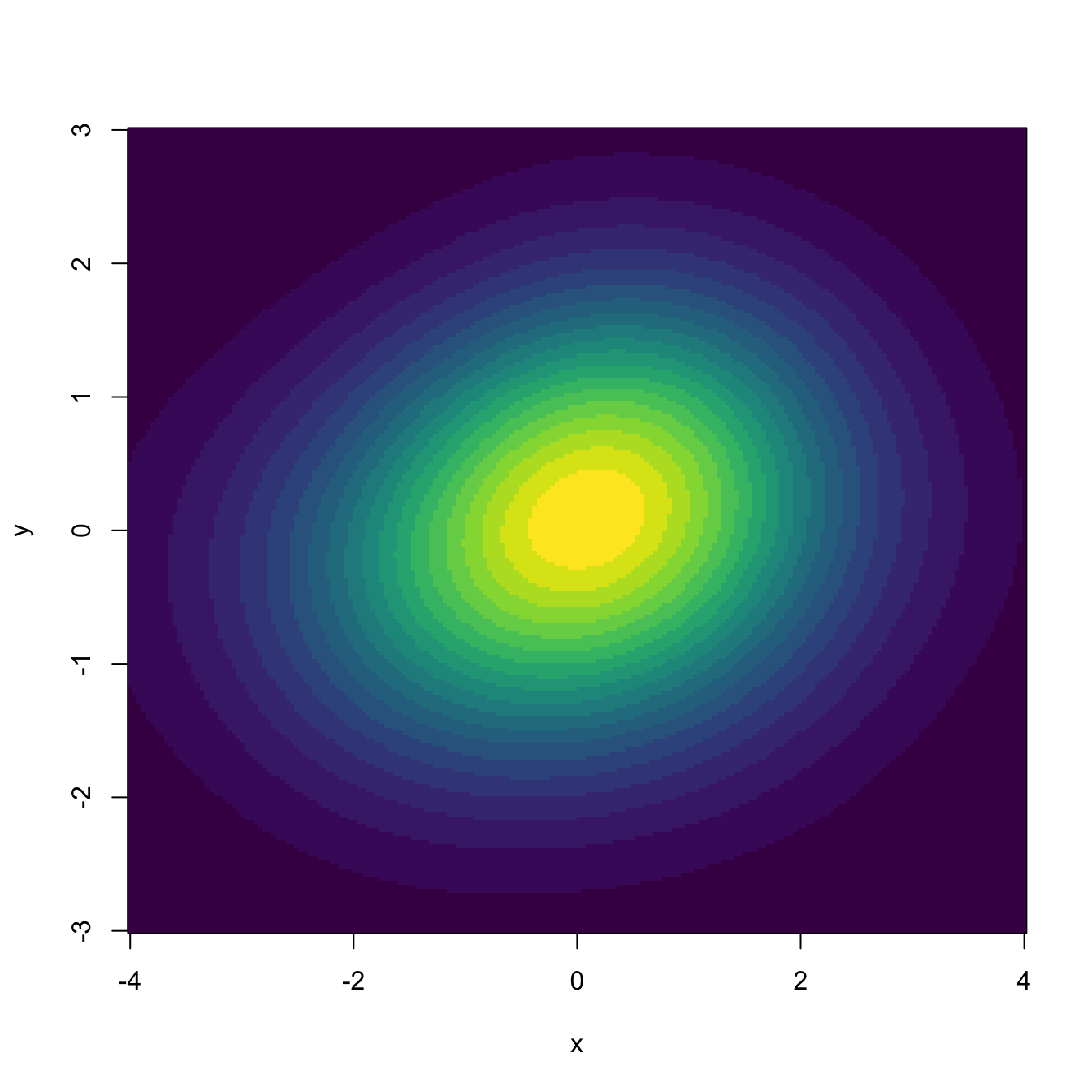
dim(kde$estimate)
## [1] 200 200

# Do not confuse "gridsize" with "bgridsize". The latter controls the internal
# grid size for binning the data and speeding up the computations (compare
# with binned = FALSE for a large sample size), and is not recommended to
# modify unless you know what you are doing. The binning takes place if
# binned = TRUE or if "binned" is not specified and the sample size is large

# Evaluating the kde at specific points can be done with "eval.points"
kde_sample <- ks::kde(x = x, H = H, eval.points = x)
str(kde_sample$estimate)
##  num [1:200] 0.0803 0.0332 0.0274 0.0739 0.0411 ...

# Assign colors automatically from quantiles to have an idea the densities of
# each one
n_cols <- 20
quantiles <- quantile(kde_sample$estimate, probs = seq(0, 1, l = n_cols + 1))
col <- viridis::viridis(n_cols)[cut(kde_sample$estimate, breaks = quantiles)]
plot(x, col = col, pch = 19, xlab = "x", ylab = "y")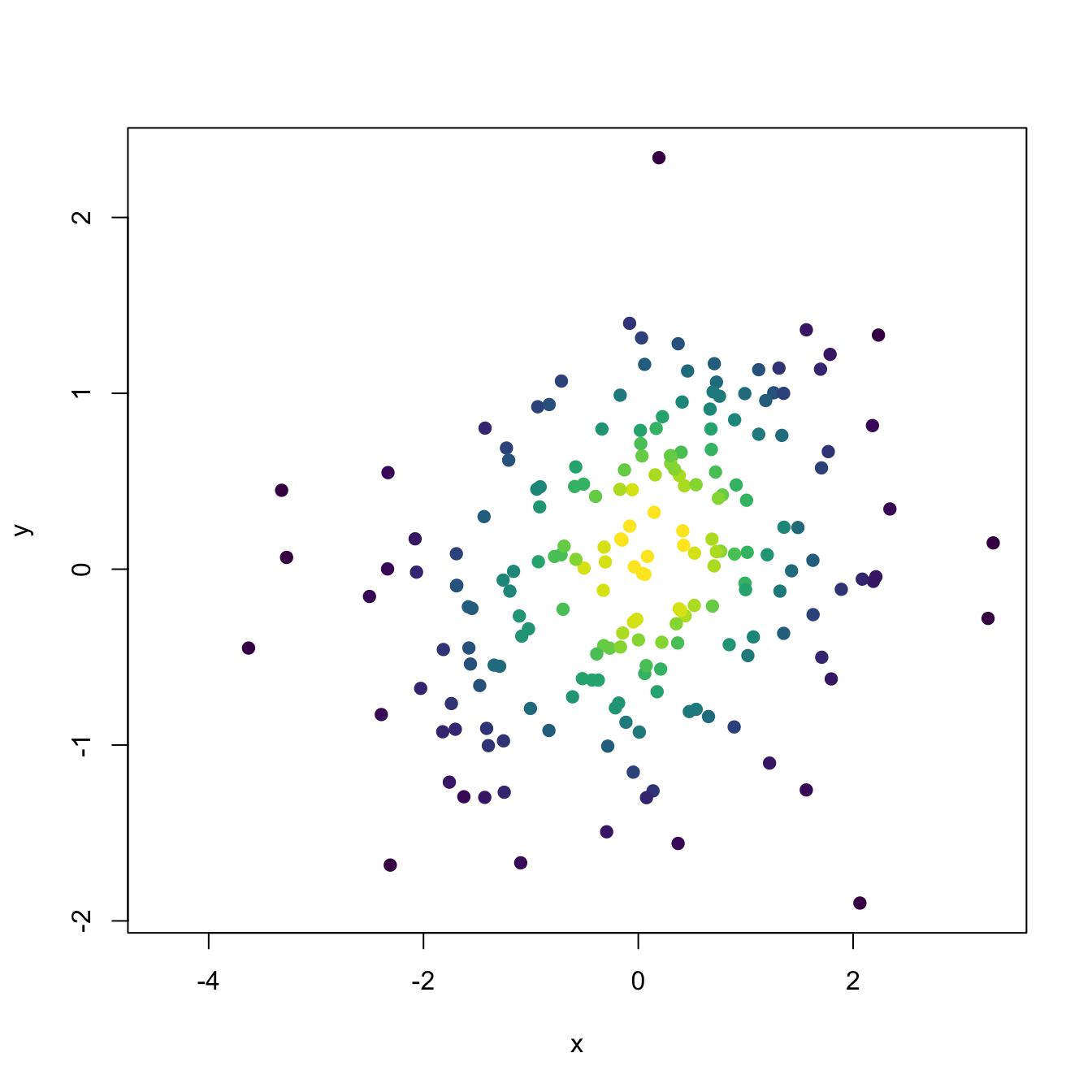
# Binning vs. not binning
abs(max(ks::kde(x = x, H = H, eval.points = x, binned = TRUE)$estimate -
          ks::kde(x = x, H = H, eval.points = x, binned = FALSE)$estimate))
## [1] 2.189159e-05
There are specific, more sophisticated, plot methods for ks::kde objects via ks::plot.kde.
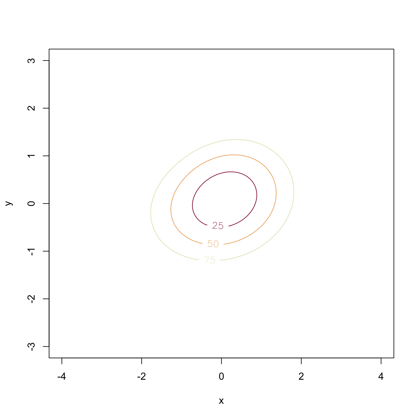
# "cont" specifies the density contours, which are upper percentages of the
# highest density regions. The default contours are at 25%, 50%, and 75%

# Raw image with custom colors
plot(kde, display = "image", xlab = "x", ylab = "y", col = viridis::viridis(20))
# Filled contour with custom color palette in "col.fun"
plot(kde, display = "filled.contour2", cont = seq(5, 95, by = 10),
     xlab = "x", ylab = "y", col.fun = viridis::viridis)
# Alternatively: col = viridis::viridis(length(cont) + 1)

# Add contourlevels
plot(kde, display = "filled.contour", cont = seq(5, 95, by = 10),
     xlab = "x", ylab = "y", col.fun = viridis::viridis)
plot(kde, display = "slice", cont = seq(5, 95, by = 10), add = TRUE)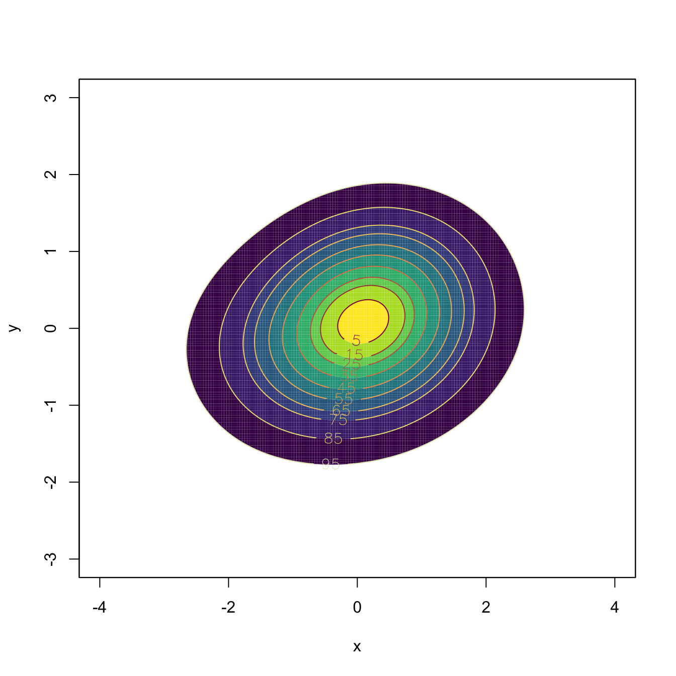
Kernel density estimation in \(\mathbb{R}^3\) can be visualized via 3D contours (to be discussed in more detail in Section 3.5.1) that represent the level surfaces.
# Simulated data from a trivariate normal
n <- 500
set.seed(213212)
x <- mvtnorm::rmvnorm(n = n, mean = c(0, 0, 0),
                      sigma = rbind(c(1.5, 0.25, 0.5),
                                    c(0.25, 0.75, 1),
                                    c(0.5, 1, 2)))

# Show nested contours of high-density regions
plot(ks::kde(x = x, H = diag(c(rep(1.25, 3)))), drawpoints = TRUE, col.pt = 1)
# Beware! Incorrect (not symmetric or positive definite) bandwidths do not
# generate an error, but they return a nonsense kde
head(ks::kde(x = x, H = diag(c(1, 1, -1)), eval.points = x)$estimate)
## [1] Inf Inf Inf Inf Inf Inf
head(ks::kde(x = x, H = diag(c(1, 1, 0)), eval.points = x)$estimate)
## [1] Inf Inf Inf Inf Inf Inf

# H not positive definite
H <- rbind(c(1.5, 0.25, 0.5),
           c(0.25, 0.75, -1.5),
           c(0.5, -1.5, 2))
eigen(H)$values
## [1]  3.0519537  1.5750921 -0.3770458
head(ks::kde(x = x, H = H, eval.points = x)$estimate)
## [1] Inf Inf Inf Inf Inf Inf

# H positive semidefinite but not positive definite
H <- rbind(c(1.5, 0.25, 0.5),
           c(0.25, 0.5, 1),
           c(0.5, 1, 2))
eigen(H)$values
## [1] 2.750000e+00 1.250000e+00 5.817207e-17
head(ks::kde(x = x, H = H, eval.points = x)$estimate) # Numerical instabilities
## [1] 10277.88 10277.88 10277.88 10277.88 10277.88 10277.88
The kde can be computed in higher dimensions (up to \(p\leq 6,\) the maximum supported by ks) with a little care to avoid a bug in versions of ks prior to 1.11.4. For these outdated versions, the bug was present in the ks::kde function for dimensions \(p\geq 4,\) as illustrated in the example below.
# Sample test data
p <- 4
data <- mvtnorm::rmvnorm(n = 10, mean = rep(0, p))
kde <- ks::kde(x = data, H = diag(rep(1, p))) # Error on the verbose argument
The bug resided in the default arguments of the internal function ks:::kde.points, and as a consequence made ks::kde not immediately usable. Although the bug has been patched since the 1.11.4 version of ks, it is interesting to observe that this and other bugs one may encounter in any function within an R package (even internal functions) can be patched in-session by means of the following code, which simply replaces a function in the environment of the loaded package.
# Create the replacement function. In this case, we just set the default
# argument of ks:::kde.points to F (FALSE)
kde.points.fixed <- function (x, H, eval.points, w, verbose = FALSE) {
  n <- nrow(x)
  d <- ncol(x)
  ne <- nrow(eval.points)
  Hs <- replicate(n, H, simplify = FALSE)
  Hs <- do.call(rbind, Hs)
  fhat <- dmvnorm.mixt(x = eval.points, mus = x, Sigmas = Hs,
                       props = w / n, verbose = verbose)
  return(list(x = x, eval.points = eval.points, estimate = fhat,
              H = H, gridded = FALSE))
}

# Assign package environment to the replacement function
environment(kde.points.fixed) <- environment(ks:::kde.points)

# Overwrite original function with replacement (careful -- you will have to
# restart session to come back to the original object)
assignInNamespace(x = "kde.points", value = kde.points.fixed, ns = "ks",
                  pos = 3)
# ns = "ks" to indicate the package namespace, pos = 3 to indicate :::

# Check the result
ks:::kde.points
Another peculiarity of ks::kde to be aware of is that it does not implement binned kde for dimension \(p>4,\) so it is necessary to set the flag binned = FALSE55 when calling ks::kde.
Observe that, if \(p=1,\) then \(\mathbf{H}\) will equal the square of the bandwidth \(h,\) that is, \(\mathbf{H}=h^2.\)↩︎
A positive definite matrix is a real symmetric matrix with positive eigenvalues. Recall that this is of key importance in order to guarantee that \(|\mathbf{H}|^{1/2}\) (\(|\mathbf{H}|\) must be nonnegative!) and \(\mathbf{H}^{-1/2}\) are well-defined (\(\mathbf{H}^{-1/2}:=\mathbf{P}\boldsymbol{\Lambda}^{1/2}\mathbf{P}'\) where \(\mathbf{H}=\mathbf{P}\boldsymbol{\Lambda}\mathbf{P}'\) is the spectral decomposition of \(\mathbf{H}\) with \(\boldsymbol{\Lambda}=\mathrm{diag}(\lambda_1,\ldots,\lambda_p)\) and \(\boldsymbol{\Lambda}^{1/2}:=\mathrm{diag}(\lambda_1^{1/2},\ldots,\lambda_p^{1/2})\)).↩︎
Beware! For the package version 1.11.3 the error message has a typo and asks to set
binned = TRUE, precisely what generated the error. This has been fixed since version 1.11.4.↩︎