6.1 Goodness-of-fit tests for distribution models

Assume that an iid sample $X_1,\ldots,X_n$ from an arbitrary distribution $F$ is given.²⁰⁰ We next address the one-sample problem of testing a statement about the unknown distribution $F.$

6.1.1 Simple hypothesis tests

We first address tests for the simple null hypothesis

$\begin{align} H_0:F=F_0 \tag{6.1} \end{align}$

against the most general alternative²⁰¹

$\begin{align*} H_1:F\neq F_0, \end{align*}$

where here and henceforth “ $F\neq F_0$ ” means that there exists at least one $x\in\mathbb{R}$ such that $F(x)\neq F_0(x),$ and $F_0$ is a pre-specified, not-data-dependent distribution model. This latter aspect is very important:

If some parameters of $F_0$ are estimated from the sample, the presented tests for (6.1) will not respect the significance level $\alpha$ for which they are constructed, and as a consequence they will be highly conservative.²⁰²

Recall that the ecdf (1.1) of $X_1,\ldots,X_n,$ $F_n(x)=\frac{1}{n}\sum_{i=1}^n1_{\{X_i\leq x\}},$ is a nonparametric estimator of $F,$ as seen in Section 1.6. Therefore, a measure of proximity of $F_n$ (driven by the sample) and $F_0$ (specified by $H_0$ ) will be indicative of the veracity of (6.1): a “large” distance between $F_n$ and $F_0$ evidences that $H_0$ is likely to be false.²⁰³ $\!\!^,$ ²⁰⁴

The following three well-known goodness-of-fit tests arise from the same principle: considering as the test statistic a particular type of distance between the functions $F_n$ and $F_0.$

Kolmogorov–Smirnov test

Test purpose. Given $X_1,\ldots,X_n\sim F,$ it tests $H_0: F=F_0$ vs. $H_1: F\neq F_0$ consistently against all the alternatives in $H_1.$
Statistic definition. The test statistic uses the supremum distance²⁰⁵ $\!\!^,$ ²⁰⁶ between $F_n$ and $F_0$ :

$\begin{align*} D_n:=\sqrt{n}\sup_{x\in\mathbb{R}} \left|F_n(x)-F_0(x)\right|. \end{align*}$

If $H_0:F=F_0$ holds, then $D_n$ tends to be small. Conversely, when $F\neq F_0,$ larger values of $D_n$ are expected, and the test rejects $H_0$ when $D_n$ is large.
Statistic computation. The computation of $D_n$ can be efficiently achieved by realizing that the maximum difference between $F_n$ and $F_0$ happens at $x=X_i,$ for a certain $X_i$ (observe Figure 6.1). From here, sorting the sample and applying the probability transformation $F_0$ gives²⁰⁷

$\begin{align} D_n=&\,\max(D_n^+,D_n^-),\tag{6.2}\\ D_n^+:=&\,\sqrt{n}\max_{1\leq i\leq n}\left\{\frac{i}{n}-U_{(i)}\right\},\nonumber\\ D_n^-:=&\,\sqrt{n}\max_{1\leq i\leq n}\left\{U_{(i)}-\frac{i-1}{n}\right\},\nonumber \end{align}$

where $U_{(j)}$ stands for the $j$ -th sorted $U_i:=F_0(X_i),$ $i=1,\ldots,n.$
Distribution under $H_0.$ If $H_0$ holds and $F_0$ is continuous, then $D_n$ has an asymptotic²⁰⁸ cdf given by the Kolmogorov–Smirnov’s $K$ ²⁰⁹ function:

$\begin{align} \lim_{n\to\infty}\mathbb{P}[D_n\leq x]=K(x):=1-2\sum_{j=1}^\infty (-1)^{j-1}e^{-2j^2x^2}.\tag{6.3} \end{align}$
Highlights and caveats. The Kolmogorov–Smirnov test is a distribution-free test because its distribution under $H_0$ does not depend on $F_0.$ However, this is the case only if $F_0$ is continuous and the sample $X_1,\ldots,X_n$ is also continuous, i.e., if the sample has no ties.²¹⁰ If these assumptions are met, then the iid sample $X_1,\ldots,X_n\stackrel{H_0}{\sim} F_0$ generates the iid sample $U_1,\ldots,U_n\stackrel{H_0}{\sim} \mathcal{U}(0,1),$ with $U_i:=F_0(X_i),$ $i=1,\ldots,n.$ As a consequence, the distribution of (6.2) does not depend on $F_0$ .²¹¹ $\!\!^,$ ²¹² If $F_0$ is not continuous or there are ties on the sample, the $K$ function is not the true asymptotic cdf. An alternative for discrete $F_0$ is given below. In case there are ties on the sample, a possibility is to slightly perturb the sample in order to remove such ties.²¹³
Implementation in R. For continuous data and continuous $F_0,$ the test statistic $D_n$ and the asymptotic $p$ -value²¹⁴ are readily available through the ks.test function. The asymptotic cdf $K\,$ is internally coded as the pkolmogorov1x function within the source code of ks.test. For discrete $F_0,$ see dgof::ks.test.

The construction of the Kolmogorov–Smirnov test statistic is illustrated in the following chunk of code.

# Sample data
n <- 10
mu0 <- 2
sd0 <- 1
set.seed(54321)
samp <- rnorm(n = n, mean = mu0, sd = sd0)

# Fn vs. F0
plot(ecdf(samp), main = "", ylab = "Probability", xlim = c(-1, 6),
     ylim = c(0, 1.3))
curve(pnorm(x, mean = mu0, sd = sd0), add = TRUE, col = 4)

# Add Dn+ and Dn-
samp_sorted <- sort(samp)
Ui <- pnorm(samp_sorted, mean = mu0, sd = sd0)
Dn_plus <- (1:n) / n - Ui
Dn_minus <- Ui - (1:n - 1) / n
i_plus <- which.max(Dn_plus)
i_minus <- which.max(Dn_minus)
lines(rep(samp_sorted[i_plus], 2), 
      c(i_plus / n, pnorm(samp_sorted[i_plus], mean = mu0, sd = sd0)), 
      col = 3, lwd = 2, pch = 16, type = "o", cex = 0.75)
lines(rep(samp_sorted[i_minus], 2), 
      c((i_minus - 1) / n, pnorm(samp_sorted[i_minus], mean = mu0, sd = sd0)), 
      col = 2, lwd = 2, pch = 16, type = "o", cex = 0.75)
rug(samp)
legend("topleft", lwd = 2, col = c(1, 4, 3, 2), 
       legend = latex2exp::TeX(c("$F_n$", "$F_0$", "$D_n^+$", "$D_n^-$")))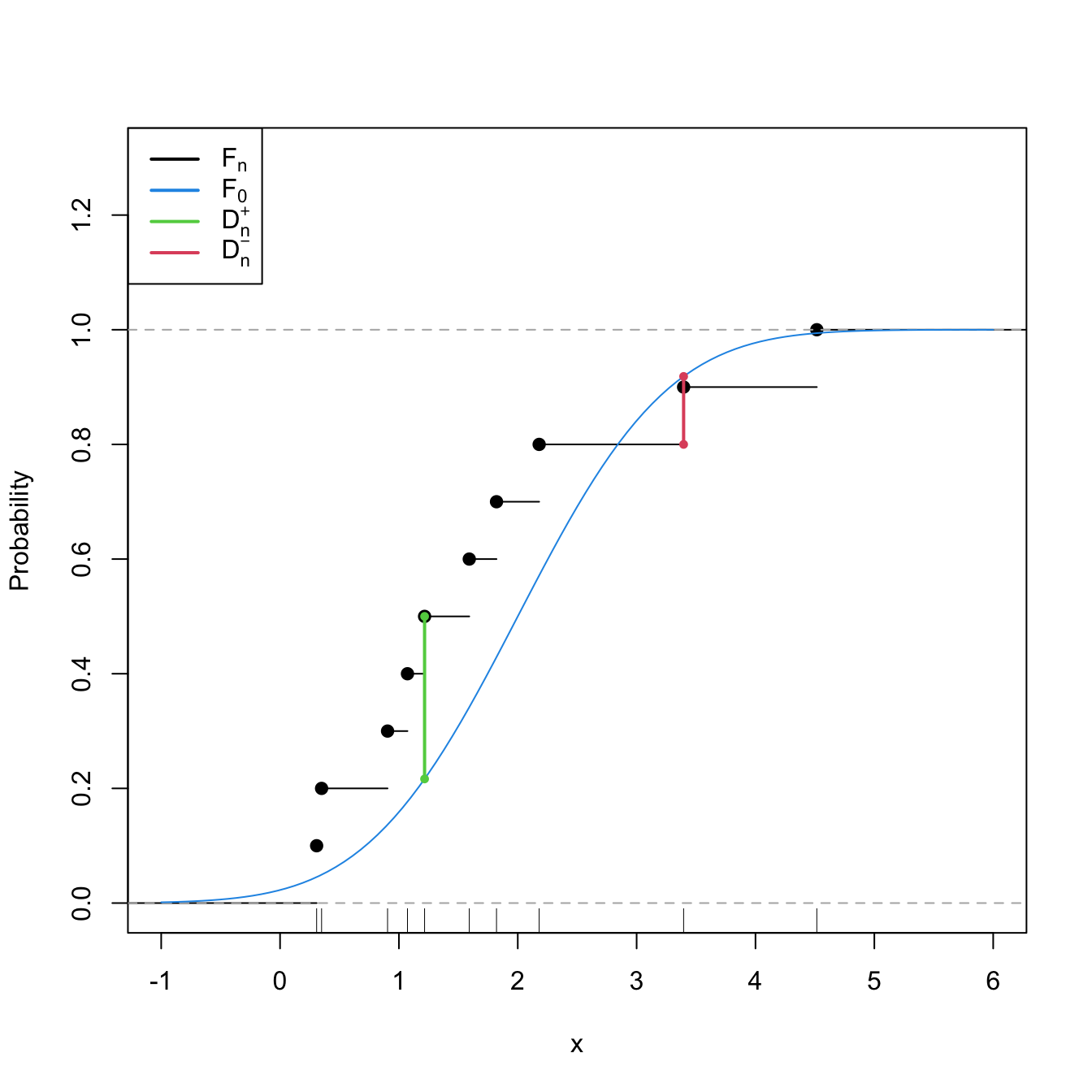

$Computation of the Kolmogorov–Smirnov statistic $D_n=\max(D_n^+,D_n^-)$ for a sample of size $n=10$ coming from $F_0(\cdot)=\Phi\left(\frac{\cdot-\mu_0}{\sigma_0}\right),$ where $\mu_0=2$ and $\sigma_0=1.$ In the example shown, $D_n=D_n^+.$$

Figure 6.1: Computation of the Kolmogorov–Smirnov statistic $D_n=\max(D_n^+,D_n^-)$ for a sample of size $n=10$ coming from $F_0(\cdot)=\Phi\left(\frac{\cdot-\mu_0}{\sigma_0}\right),$ where $\mu_0=2$ and $\sigma_0=1.$ In the example shown, $D_n=D_n^+.$

Exercise 6.1 Modify if the parameters mu0 and sd0 in the previous code in order to have $F\neq F_0.$ What happens with $\sup_{x\in\mathbb{R}} \left|F_n(x)-F_0(x)\right|$ ?

Let’s see an example of the use of ks.test (also available as stats::ks.test), the function in base R.

# Sample data from a N(0, 1)
n <- 50
set.seed(3245678)
x <- rnorm(n = n)

# Kolmogorov-Smirnov test for H_0: F = N(0, 1). Does not reject
(ks <- ks.test(x = x, y = "pnorm")) # In "y" we specify F0 as a function
## 
##  Exact one-sample Kolmogorov-Smirnov test
## 
## data:  x
## D = 0.050298, p-value = 0.9989
## alternative hypothesis: two-sided

# Structure of "htest" class
str(ks)
## List of 7
##  $ statistic  : Named num 0.0503
##   ..- attr(*, "names")= chr "D"
##  $ p.value    : num 0.999
##  $ alternative: chr "two-sided"
##  $ method     : chr "Exact one-sample Kolmogorov-Smirnov test"
##  $ data.name  : chr "x"
##  $ data       :List of 2
##   ..$ x: num [1:50] 0.01911 0.0099 -0.01005 -0.02856 0.00282 ...
##   ..$ y:function (q, mean = 0, sd = 1, lower.tail = TRUE, log.p = FALSE)  
##  $ exact      : logi TRUE
##  - attr(*, "class")= chr [1:2] "ks.test" "htest"

# Kolmogorov-Smirnov test for H_0: F = N(0.5, 1). Rejects
ks.test(x = x, y = "pnorm", mean = 0.5)
## 
##  Exact one-sample Kolmogorov-Smirnov test
## 
## data:  x
## D = 0.24708, p-value = 0.003565
## alternative hypothesis: two-sided

# Kolmogorov-Smirnov test for H_0: F = Exp(2). Strongly rejects
ks.test(x = x, y = "pexp", rate = 1/2)
## 
##  Exact one-sample Kolmogorov-Smirnov test
## 
## data:  x
## D = 0.53495, p-value = 6.85e-14
## alternative hypothesis: two-sided

The following chunk of code shows how to call dgof::ks.test to perform a correct Kolmogorov–Smirnov when $F_0$ is discrete.

# Sample data from a Pois(5)
n <- 100
set.seed(3245678)
x <- rpois(n = n, lambda = 5)

# Kolmogorov-Smirnov test for H_0: F = Pois(5) without specifying that the 
# distribution is discrete. Rejects (!?) giving a warning message
ks.test(x = x, y = "ppois", lambda = 5)
## 
##  Asymptotic one-sample Kolmogorov-Smirnov test
## 
## data:  x
## D = 0.20596, p-value = 0.0004135
## alternative hypothesis: two-sided

# We rely on dgof::ks.test, which works as stats::ks.test if the "y" argument 
# is not marked as a "stepfun" object, the way the dgof package codifies
# discrete distribution functions

# Step function containing the cdf of the Pois(5). The "x" stands for the 
# location of the steps and "y" for the value of the steps. "y" needs to have
# an extra point for the initial value of the function before the first step
x_eval <- 0:20
ppois_stepfun <- stepfun(x = x_eval, y = c(0, ppois(q = x_eval, lambda = 5)))
plot(ppois_stepfun, main = "Cdf of a Pois(5)")


# Kolmogorov-Smirnov test for H_0: F = Pois(5) adapted for discrete data,
# with data coming from a Pois(5)
dgof::ks.test(x = x, y = ppois_stepfun)
## 
##  One-sample Kolmogorov-Smirnov test
## 
## data:  x
## D = 0.032183, p-value = 0.9999
## alternative hypothesis: two-sided

# If data is normally distributed, the test rejects H_0
dgof::ks.test(x = rnorm(n = n, mean = 5), y = ppois_stepfun)
## 
##  One-sample Kolmogorov-Smirnov test
## 
## data:  rnorm(n = n, mean = 5)
## D = 0.38049, p-value = 5.321e-13
## alternative hypothesis: two-sided

Exercise 6.2 Implement the Kolmogorov–Smirnov test by:

Coding a function to compute the test statistic (6.2) from a sample $X_1,\ldots,X_n$ and a cdf $F_0.$
Implementing the $K$ function (6.3).
Calling the previous functions from a routine that returns the asymptotic $p$ -value of the test.

Check that the implementations coincide with the ones of the ks.test function when exact = FALSE for data simulated from a $\mathcal{U}(0,1)$ and any $n.$ Note: ks.test computes $D_n/\sqrt{n}$ instead of $D_n.$

The following code chunk exemplifies with a small simulation study how the distribution of the $p$ -values²¹⁵ is uniform if $H_0$ holds, and how it becomes more concentrated about $0$ when $H_1$ holds.

# Simulation of p-values when H_0 is true
set.seed(131231)
n <- 100
M <- 1e4
pvalues_H0 <- sapply(1:M, function(i) {
  x <- rnorm(n) # N(0, 1)
  ks.test(x, "pnorm")$p.value
})

# Simulation of p-values when H_0 is false -- the data does not
# come from a N(0, 1) but from a N(0, 2)
pvalues_H1 <- sapply(1:M, function(i) {
  x <- rnorm(n, mean = 0, sd = sqrt(2)) # N(0, 2)
  ks.test(x, "pnorm")$p.value
})

# Comparison of p-values
par(mfrow = 1:2)
hist(pvalues_H0, breaks = seq(0, 1, l = 20), probability = TRUE,
     main = latex2exp::TeX("$H_0$"), ylim = c(0, 10))
abline(h = 1, col = 2)
hist(pvalues_H1, breaks = seq(0, 1, l = 20), probability = TRUE,
     main = latex2exp::TeX("$H_1$"), ylim = c(0, 10))
abline(h = 1, col = 2)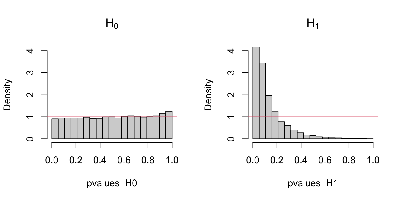

$Comparison of the distribution of $p$-values under $H_0$ and $H_1$ for the Kolmogorov–Smirnov test. Observe that the frequency of low $p$-values, associated with the rejection of $H_0,$ increases when $H_0$ does not hold. Under $H_0,$ the distribution of the $p$-values is uniform.$

Figure 6.2: Comparison of the distribution of $p$ -values under $H_0$ and $H_1$ for the Kolmogorov–Smirnov test. Observe that the frequency of low $p$ -values, associated with the rejection of $H_0,$ increases when $H_0$ does not hold. Under $H_0,$ the distribution of the $p$ -values is uniform.

Exercise 6.3 Modify the parameters of the normal distribution used to sample under $H_1$ in order to increase and decrease the deviation from $H_0.$ What do you observe in the resulting distributions of the $p$ -values?

Cramér–von Mises test

Test purpose. Given $X_1,\ldots,X_n\sim F,$ it tests $H_0: F=F_0$ vs. $H_1: F\neq F_0$ consistently against all the alternatives in $H_1.$
Statistic definition. The test statistic uses a quadratic distance²¹⁶ between $F_n$ and $F_0$ :

$\begin{align} W_n^2:=n\int(F_n(x)-F_0(x))^2\,\mathrm{d}F_0(x).\tag{6.4} \end{align}$

If $H_0: F=F_0$ holds, then $W_n^2$ tends to be small. Hence, rejection happens for large values of $W_n^2.$
Statistic computation. The computation of $W_n^2$ can be significantly simplified by expanding the square in the integrand of (6.4) and then applying the change of variables $u=F_0(x)$ :

$\begin{align} W_n^2=\sum_{i=1}^n\left\{U_{(i)}-\frac{2i-1}{2n}\right\}^2+\frac{1}{12n},\tag{6.5} \end{align}$

where again $U_{(j)}$ stands for the $j$ -th sorted $U_i=F_0(X_i),$ $i=1,\ldots,n.$
Distribution under $H_0.$ If $H_0$ holds and $F_0$ is continuous, then $W_n^2$ has an asymptotic cdf given by²¹⁷

$\begin{align} \lim_{n\to\infty}\mathbb{P}[W_n^2\leq x]=&\,1-\frac{1}{\pi}\sum_{j=1}^\infty (-1)^{j-1}W_j(x),\tag{6.6}\\ W_j(x):=&\,\int_{(2j-1)^2\pi^2}^{4j^2\pi^2}\sqrt{\frac{-\sqrt{y}}{\sin\sqrt{y}}}\frac{e^{-\frac{xy}{2}}}{y}\,\mathrm{d}y.\nonumber \end{align}$
Highlights and caveats. By a reasoning analogous to the one done in the Kolmogorov–Smirnov test, the Cramér–von Mises test can be seen to be distribution-free if $F_0$ is continuous and the sample has no ties. Otherwise, (6.6) is not the true asymptotic distribution. Although the Kolmogorov–Smirnov test is the most popular ecdf-based test, empirical evidence suggests that the Cramér–von Mises test is often more powerful than the Kolmogorov–Smirnov test for a broad class of alternative hypotheses.²¹⁸
Implementation in R. For continuous data, the test statistic $W_n^2$ and the asymptotic $p$ -value are implemented in the goftest::cvm.test function. The asymptotic cdf (6.6) is given in goftest::pCvM (goftest::qCvM computes its inverse). For discrete $F_0,$ see dgof::cvm.test.

The following chunk of code points to the implementation of the Cramér–von Mises test.

# Sample data from a N(0, 1)
set.seed(3245678)
n <- 50
x <- rnorm(n = n)

# Cramér-von Mises test for H_0: F = N(0, 1). Does not reject
goftest::cvm.test(x = x, null = "pnorm")
## 
##  Cramer-von Mises test of goodness-of-fit
##  Null hypothesis: Normal distribution
##  Parameters assumed to be fixed
## 
## data:  x
## omega2 = 0.022294, p-value = 0.9948

# Comparison with Kolmogorov-Smirnov
ks.test(x = x, y = "pnorm") 
## 
##  Exact one-sample Kolmogorov-Smirnov test
## 
## data:  x
## D = 0.050298, p-value = 0.9989
## alternative hypothesis: two-sided

# Sample data from a Pois(5)
set.seed(3245678)
n <- 100
x <- rpois(n = n, lambda = 5)

# Cramér-von Mises test for H_0: F = Pois(5) without specifying that the 
# distribution is discrete. Rejects (!?) without giving a warning message
goftest::cvm.test(x = x, null = "ppois", lambda = 5)
## 
##  Cramer-von Mises test of goodness-of-fit
##  Null hypothesis: Poisson distribution
##  with parameter lambda = 5
##  Parameters assumed to be fixed
## 
## data:  x
## omega2 = 0.74735, p-value = 0.009631

# We rely on dgof::cvm.test and run a Cramér-von Mises test for H_0: F = Pois(5)
# adapted for discrete data, with data coming from a Pois(5)
x_eval <- 0:20
ppois_stepfun <- stepfun(x = x_eval, y = c(0, ppois(q = x_eval, lambda = 5)))
dgof::cvm.test(x = x, y = ppois_stepfun)
## 
##  Cramer-von Mises - W2
## 
## data:  x
## W2 = 0.038256, p-value = 0.9082
## alternative hypothesis: Two.sided

# Plot the asymptotic null distribution function
curve(goftest::pCvM(x), from = 0, to = 1, n = 300)

Exercise 6.4 Implement the Cramér–von Mises test by:

Coding the Cramér–von Mises statistic (6.5) from a sample $X_1,\ldots,X_n$ and a cdf $F_0.$ Check that the implementation coincides with the one of the goftest::cvm.test function.
Computing the asymptotic $p$ -value using goftest::pCvM. Compare this asymptotic $p$ -value with the exact $p$ -value given by goftest::cvm.test, observing that for a large $n$ the difference is inappreciable.

Exercise 6.5 Verify the correctness of the asymptotic null distribution of $W_n^2$ that was given in (6.6). To do so, numerically implement $W_j(x)$ and compute (6.6). Validate your implementation by:

Simulating $M=1,000$ samples of size $n=200$ under $H_0,$ obtaining $M$ statistics $W_{n;1}^{2},\ldots, W_{n;M}^{2},$ and plotting their ecdf.
Overlaying your asymptotic cdf and the one provided by goftest::pCvM.
Checking that the three curves approximately coincide.

Anderson–Darling test

Test purpose. Given $X_1,\ldots,X_n\sim F,$ it tests $H_0: F=F_0$ vs. $H_1: F\neq F_0$ consistently against all the alternatives in $H_1.$
Statistic definition. The test statistic uses a quadratic distance between $F_n$ and $F_0$ weighted by $w(x)=(F_0(x)(1-F_0(x)))^{-1}$ :

$\begin{align*} A_n^2:=n\int\frac{(F_n(x)-F_0(x))^2}{F_0(x)(1-F_0(x))}\,\mathrm{d}F_0(x). \end{align*}$

If $H_0$ holds, then $A_n^2$ tends to be small (because of the denominator). Hence, rejection happens for large values of $A_n^2.$ Note that, compared with $W_n^2,$ $A_n^2$ places more weight on the deviations between $F_n(x)$ and $F_0(x)$ that happen on the tails, that is, when $F_0(x)\approx 0$ or $F_0(x)\approx 1.$ ²¹⁹ $\!\!^,$ ²²⁰
Statistic computation. The computation of $A_n^2$ can be significantly simplified:

$\begin{align} A_n^2=-n-\frac{1}{n}\sum_{i=1}^n&\Big\{(2i-1)\log(U_{(i)})\nonumber\\ &+(2n+1-2i)\log(1-U_{(i)})\Big\}.\tag{6.7} \end{align}$
Distribution under $H_0.$ If $H_0$ holds and $F_0$ is continuous, then the asymptotic cdf of $A_n^2$ is the cdf of the random variable

$\begin{align} \sum_{j=1}^\infty\frac{Y_j}{j(j+1)},\quad \text{where } Y_j\sim\chi^2_1,\,j\geq 1,\text{ are iid}.\tag{6.8} \end{align}$

Unfortunately, the cdf of (6.8) does not admit a simple analytical expression. It can, however, be approximated by Monte Carlo by sampling from the random variable (6.8).
Highlights and caveats. As with the previous tests, the Anderson–Darling test is also distribution-free if $F_0$ is continuous and there are no ties in the sample. Otherwise, the null asymptotic distribution is different from the one of (6.8). As for the Cramér–von Mises test, there is also empirical evidence indicating that the Anderson–Darling test is more powerful than the Kolmogorov–Smirnov test for a broad class of alternative hypotheses. In addition, due to its construction, the Anderson–Darling test is able to detect better the situations in which $F_0$ and $F$ differ on the tails (that is, for extreme data).
Implementation in R. For continuous data, the test statistic $A_n^2$ and the asymptotic $p$ -value are implemented in the goftest::ad.test function. The asymptotic cdf of (6.8) is given in goftest::pAD (goftest::qAD computes its inverse). For discrete $F_0,$ see dgof::cvm.test with type = "A2".

The following code chunk illustrates the implementation of the Anderson–Darling test.

# Sample data from a N(0, 1)
set.seed(3245678)
n <- 50
x <- rnorm(n = n)

# Anderson-Darling test for H_0: F = N(0, 1). Does not reject
goftest::ad.test(x = x, null = "pnorm")
## 
##  Anderson-Darling test of goodness-of-fit
##  Null hypothesis: Normal distribution
##  Parameters assumed to be fixed
## 
## data:  x
## An = 0.18502, p-value = 0.994

# Sample data from a Pois(5)
set.seed(3245678)
n <- 100
x <- rpois(n = n, lambda = 5)

# Anderson-Darling test for H_0: F = Pois(5) without specifying that the 
# distribution is discrete. Rejects (!?) without giving a warning message
goftest::ad.test(x = x, null = "ppois", lambda = 5)
## 
##  Anderson-Darling test of goodness-of-fit
##  Null hypothesis: Poisson distribution
##  with parameter lambda = 5
##  Parameters assumed to be fixed
## 
## data:  x
## An = 3.7279, p-value = 0.01191

# We rely on dgof::cvm.test and run an Anderson-Darling test for H_0: F = Pois(5)
# adapted for discrete data, with data coming from a Pois(5)
x_eval <- 0:20
ppois_stepfun <- stepfun(x = x_eval, y = c(0, ppois(q = x_eval, lambda = 5)))
dgof::cvm.test(x = x, y = ppois_stepfun, type = "A2")
## 
##  Cramer-von Mises - A2
## 
## data:  x
## A2 = 0.3128, p-value = 0.9057
## alternative hypothesis: Two.sided

# Plot the asymptotic null distribution function
curve(goftest::pAD(x), from = 0, to = 5, n = 300)

Exercise 6.6 Implement the Anderson–Darling test by:

Coding the Anderson–Darling statistic (6.7) from a sample $X_1,\ldots,X_n$ and a cdf $F_0.$ Check that the implementation coincides with the one of the goftest::ad.test function.
Computing the asymptotic $p$ -value using goftest::pAD. Compare this asymptotic $p$ -value with the exact $p$ -value given by goftest::ad.test, observing that for large $n$ the difference is inappreciable.

Exercise 6.7 Verify the correctness of the asymptotic representation of $A_n^2$ that was given in (6.8). To do so:

Simulate $M=1,000$ samples of size $n=200$ under $H_0,$ obtain $M$ statistics $A_{n;1}^{2},\ldots, A_{n;M}^{2},$ and draw its histogram.
Simulate $M$ samples from the random variable (6.8) and draw its histogram.
Check that the two histograms approximately coincide.

Exercise 6.8 Let’s investigate empirically the performance of the Kolmogorov–Smirnov, Cramér–von Mises, and Anderson–Darling tests for a specific scenario. We consider $H_0:X\sim \mathcal{N}(0,1)$ and the following simulation study:

Generate $M=1,000$ samples of size $n$ from $\mathcal{N}(\mu,1).$
For each sample, test $H_0$ with the three tests.
Obtain the relative frequency of rejections at level $\alpha$ for each test.
Draw three histograms for the $p$ -values in the spirit of Figure 6.3.

In order to cleanly perform the previous steps for several choices of $(n,\mu,\alpha),$ code a function that performs the simulation study from those arguments and gives something similar to Figure 6.3 as output. Then, use the following settings and accurately comment on the outcome of each of them:

$H_0$ holds.
- Take $n=25,$ $\mu=0,$ and $\alpha=0.05.$ Check that the relative frequency of rejections is about $\alpha.$
- Take $n=25,$ $\mu=0,$ and $\alpha=0.10.$
- Take $n=100,$ $\mu=0,$ and $\alpha=0.10.$
$H_0$ does not hold.
- $n=25,$ $\mu=0.25,$ $\alpha=0.05.$ Check that the relative frequency of rejections is above $\alpha.$
- $n=50,$ $\mu=0.25,$ $\alpha=0.05.$
- $n=25,$ $\mu=0.50,$ $\alpha=0.05.$
- Replace $\mathcal{N}(\mu,1)$ with $t_{10}.$ Take $n=50$ and $\alpha=0.05.$ Which test is clearly better? Why?

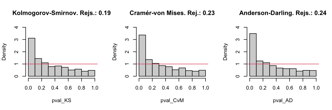
$The histograms of the $p$-values and the relative rejection frequencies for the Kolmogorov–Smirnov, Cramér–von Mises, and Anderson–Darling tests. The null hypothesis is $H_0:X\sim \mathcal{N}(0,1)$ and the sample of size $n=25$ is generated from a $\mathcal{N}(0.25,1).$ The significance level is $\alpha=0.05$.$

Figure 6.3: The histograms of the $p$ -values and the relative rejection frequencies for the Kolmogorov–Smirnov, Cramér–von Mises, and Anderson–Darling tests. The null hypothesis is $H_0:X\sim \mathcal{N}(0,1)$ and the sample of size $n=25$ is generated from a $\mathcal{N}(0.25,1).$ The significance level is $\alpha=0.05$ .

6.1.2 Normality tests

The tests seen in the previous section have a very notable practical limitation: they require complete knowledge of $F_0,$ the hypothesized distribution for $X.$ In practice, such a precise knowledge about $X$ is unrealistic. Practitioners are more interested in answering more general questions, one of them being:

Is the data “normally distributed”?

With the statement “ $X$ is normally distributed” we refer to the fact that $X\sim \mathcal{N}(\mu,\sigma^2)$ for certain parameters $\mu\in\mathbb{R}$ and $\sigma\in\mathbb{R^+},$ possibly unknown. This statement is notably more general than “ $X$ is distributed as a $\mathcal{N}(0,1)$ ” or “ $X$ is distributed as a $\mathcal{N}(0.1,1.3)$ ”.

The test for normality is formalized as follows. Given an iid sample $X_1,\ldots,X_n$ from the distribution $F,$ we test the null hypothesis

$\begin{align} H_0:F\in\mathcal{F}_{\mathcal{N}}:=\left\{\Phi\left(\frac{\cdot-\mu}{\sigma}\right):\mu\in\mathbb{R},\sigma\in\mathbb{R}^+\right\},\tag{6.9} \end{align}$

where $\mathcal{F}_{\mathcal{N}}$ is the class of normal distributions, against the most general alternative

$\begin{align*} H_1:F\not\in\mathcal{F}_{\mathcal{N}}. \end{align*}$

Comparing (6.9) with (6.1), it is evident that the former is more general, as a range of possible values for $F$ is included in $H_0.$ This is the reason why $H_0$ is called a composite null hypothesis, rather than a simple null hypothesis, as (6.1) was.

The testing of (6.9) requires the estimation of the unknown parameters $(\mu,\sigma).$ Their maximum likelihood estimators are $(\bar{X},S),$ where $S:=\sqrt{\frac{1}{n}\sum_{i=1}^n(X_i-\bar{X})^2}$ is the sample standard deviation Therefore, a tempting possibility is to apply the tests seen in Section 6.1.1 to

$\begin{align*} H_0:F=\Phi\left(\frac{\cdot-\bar{X}}{S}\right). \end{align*}$

However, as warned at the beginning of Section 6.1, this naive approach would result in seriously conservative tests that would fail to reject $H_0$ adequately. The intuitive explanation is simple: when estimating $(\mu,\sigma)$ from the sample we are obtaining the closest normal cdf to $F,$ that is, $\Phi\left(\frac{\cdot-\bar{X}}{S}\right).$ Therefore, setting $F_0=\Phi\left(\frac{\cdot-\bar{X}}{S}\right)$ and then running one of the ecdf-based tests on $H_0:F=F_0$ will ignore this estimation step, which will bias the test decision towards $H_0$ .

Adequately accounting for the estimation of $(\mu,\sigma)$ amounts to study the asymptotic distributions under $H_0$ of the test statistics that are computed with the data-dependent cdf $\Phi\left(\frac{\cdot-\bar{X}}{S}\right)$ in the place of $F_0.$ This is what is precisely done by the tests that adapt the ecdf-based tests seen in Section 6.1.1 by

replacing $F_0$ with $\Phi\left(\frac{\cdot-\bar{X}}{S}\right)$ in the formulation of the test statistics;
replacing $U_i$ with $P_i:=\Phi\left(\frac{X_i-\bar{X}}{\hat{S}}\right),$ $i=1,\ldots,n,$ in the computational forms of the statistics;²²¹
obtaining a different null asymptotic distribution that is usually more convoluted and is approximated by tabulation or simulation.

Lilliefors test (Kolmogorov–Smirnov test for normality)

Test purpose. Given $X_1,\ldots,X_n,$ it tests $H_0: F\in\mathcal{F}_\mathcal{N}$ vs. $H_1: F\not\in\mathcal{F}_\mathcal{N}$ consistently against all the alternatives in $H_1.$
Statistic definition and computation. The test statistic uses the supremum distance between $F_n$ and $\Phi\left(\frac{\cdot-\bar{X}}{S}\right)$ :

$\begin{align*} D_n=&\,\sqrt{n}\sup_{x\in\mathbb{R}} \left|F_n(x)-\Phi\left(\frac{x-\bar{X}}{S}\right)\right|=\max(D_n^+,D_n^-),\\ D_n^+=&\,\sqrt{n}\max_{1\leq i\leq n}\left\{\frac{i}{n}-P_{(i)}\right\},\\ D_n^-=&\,\sqrt{n}\max_{1\leq i\leq n}\left\{P_{(i)}-\frac{i-1}{n}\right\}, \end{align*}$

where $P_{(j)}$ stands for the $j$ -th sorted $P_i=\Phi\left(\frac{X_i-\bar{X}}{S}\right),$ $i=1,\ldots,n.$ Clearly, if $H_0$ holds, then $D_n$ tends to be small. Hence, rejection happens when $D_n$ is large.
Distribution under $H_0.$ If $H_0$ holds, the critical values at level of significance $\alpha$ can be obtained from Lilliefors (1967).²²² Dallal and Wilkinson (1986) provides an analytical approximation to the null distribution.
Highlights and caveats. The Lilliefors test is not distribution-free, in the sense that the null distribution of the test statistic clearly depends on the normality assumption. However, it is parameter-free, since the distribution does not depend on the actual parameters $(\mu,\sigma)$ for which $F=\Phi\left(\frac{\cdot-\mu}{\sigma}\right)$ is satisfied. This result comes from the iid sample $X_1,\ldots,X_n\stackrel{H_0}{\sim} \mathcal{N}(\mu,\sigma^2)$ generating the id sample $\frac{X_1-\bar{X}}{S},\ldots,\frac{X_n-\bar{X}}{S}\stackrel{H_0}{\sim} \tilde{f}_0,$ where $\tilde{f}_0$ is a certain pdf that does not depend on $(\mu,\sigma).$ ²²³ Therefore, $P_1,\ldots,P_n$ is an id sample that does not depend on $(\mu,\sigma).$
Implementation in R. The nortest::lillie.test function implements the test.

Cramér–von Mises normality test

Test purpose. Given $X_1,\ldots,X_n,$ it tests $H_0: F\in\mathcal{F}_\mathcal{N}$ vs. $H_1: F\not\in\mathcal{F}_\mathcal{N}$ consistently against all the alternatives in $H_1.$
Statistic definition and computation. The test statistic uses the quadratic distance between $F_n$ and $\Phi\left(\frac{\cdot-\bar{X}}{S}\right)$ :

$\begin{align*} W_n^2=&\,n\int\left(F_n(x)-\Phi\left(\frac{x-\bar{X}}{S}\right)\right)^2\,\mathrm{d}\Phi\left(\frac{x-\bar{X}}{S}\right)\\ =&\,\sum_{i=1}^n\left\{P_{(i)}-\frac{2i-1}{2n}\right\}^2+\frac{1}{12n}, \end{align*}$

where $P_{(j)}$ stands for the $j$ -th sorted $P_i=\Phi\left(\frac{X_i-\bar{X}}{S}\right),$ $i=1,\ldots,n.$ Rejection happens when $W_n^2$ is large.
Distribution under $H_0.$ If $H_0$ holds, the $p$ -values of the test can be approximated using Table 4.9 in D’Agostino and Stephens (1986).
Highlights and caveats. Like the Lilliefors test, the Cramér–von Mises test is also parameter-free. Its usual power superiority over the Kolmogorov–Smirnov also extends to the testing of normality.
Implementation in R. The nortest::cvm.test function implements the test.

Anderson–Darling normality test

Test purpose. Given $X_1,\ldots,X_n,$ it tests $H_0: F\in\mathcal{F}_\mathcal{N}$ vs. $H_1: F\not\in\mathcal{F}_\mathcal{N}$ consistently against all the alternatives in $H_1.$
Statistic definition and computation. The test statistic uses a weighted quadratic distance between $F_n$ and $\Phi\left(\frac{\cdot-\bar{X}}{S}\right)$ :

$\begin{align*} A_n^2=&\,n\int\frac{\left(F_n(x)-\Phi\left(\frac{x-\bar{X}}{S}\right)\right)^2}{\Phi\left(\frac{x-\bar{X}}{S}\right)\left(1-\Phi\left(\frac{x-\bar{X}}{S}\right)\right)}\,\mathrm{d}\Phi\left(\frac{x-\bar{X}}{S}\right)\\ =&\,-n-\frac{1}{n}\sum_{i=1}^n\left\{(2i-1)\log(P_{(i)})+(2n+1-2i)\log(1-P_{(i)})\right\}. \end{align*}$

Rejection happens when $A_n^2$ is large.
Distribution under $H_0.$ If $H_0$ holds, the $p$ -values of the test can be approximated using Table 4.9 in D’Agostino and Stephens (1986).
Highlights and caveats. The test is also parameter-free. Since the test statistic places more weight on the tails than the Cramér–von Mises, it is better suited for detecting heavy-tailed deviations from normality.
Implementation in R. The nortest::ad.test function implements the test.

The following code chunk gives the implementation of these normality tests.

# Sample data from a N(10, 1)
set.seed(123456)
n <- 100
x <- rnorm(n = n, mean = 10)

# Normality tests -- do not reject H0
nortest::lillie.test(x = x)
## 
##  Lilliefors (Kolmogorov-Smirnov) normality test
## 
## data:  x
## D = 0.054535, p-value = 0.6575
nortest::cvm.test(x = x)
## 
##  Cramer-von Mises normality test
## 
## data:  x
## W = 0.032898, p-value = 0.8027
nortest::ad.test(x = x)
## 
##  Anderson-Darling normality test
## 
## data:  x
## A = 0.22888, p-value = 0.8052

# Sample data from a Student's t with 3 degrees of freedom
x <- rt(n = n, df = 3)

# Normality tests -- reject H0
nortest::lillie.test(x = x)
## 
##  Lilliefors (Kolmogorov-Smirnov) normality test
## 
## data:  x
## D = 0.08453, p-value = 0.07499
nortest::cvm.test(x = x)
## 
##  Cramer-von Mises normality test
## 
## data:  x
## W = 0.19551, p-value = 0.005965
nortest::ad.test(x = x)
## 
##  Anderson-Darling normality test
## 
## data:  x
## A = 1.2842, p-value = 0.002326

# Flawed normality tests -- do not reject because the null distribution
# that is employed is wrong!
ks.test(x = x, y = "pnorm", mean = mean(x), sd = sd(x))
## 
##  Asymptotic one-sample Kolmogorov-Smirnov test
## 
## data:  x
## D = 0.08453, p-value = 0.4725
## alternative hypothesis: two-sided
goftest::cvm.test(x = x, null = "pnorm", mean = mean(x), sd = sd(x))
## 
##  Cramer-von Mises test of goodness-of-fit
##  Null hypothesis: Normal distribution
##  with parameters mean = 0.0151268546198777, sd = 1.33709561396292
##  Parameters assumed to be fixed
## 
## data:  x
## omega2 = 0.19551, p-value = 0.2766
goftest::ad.test(x = x, null = "pnorm", mean = mean(x), sd = sd(x))
## 
##  Anderson-Darling test of goodness-of-fit
##  Null hypothesis: Normal distribution
##  with parameters mean = 0.0151268546198777, sd = 1.33709561396292
##  Parameters assumed to be fixed
## 
## data:  x
## An = 1.2842, p-value = 0.2375

Shapiro–Francia normality test

We now consider a different normality test that is not based on the ecdf, the Shapiro–Francia normality test. This test is a modification of the wildly popular Shapiro–Wilk test, but the Shapiro–Francia test is easier to interpret and explain.²²⁴

The test is based on the QQ-plot of the sample $X_1,\ldots,X_n.$ The plot is comprised of the pairs $\left(\Phi^{-1}\left(\frac{i}{n+1}\right),X_{(i)}\right)\,,$ for $i=1,\ldots,n.$ ²²⁵ That is, the QQ-plot plots $\mathcal{N}(0,1)$ -quantiles against sample quantiles.

Since the $\alpha$ -lower quantile of a $\mathcal{N}(\mu,\sigma^2),$ $z_{\alpha;\mu,\sigma},$ verifies that

$\begin{align} z_{\alpha;\mu,\sigma}=\mu+\sigma z_{\alpha;0,1},\tag{6.10} \end{align}$

then, if the sample is distributed as a $\mathcal{N}(\mu,\sigma^2),$ the points of the QQ-plot are expected to align about the straight line (6.10). This is illustrated in the code below.

n <- 100
mu <- 10
sigma <- 2
set.seed(12345678)
x <- rnorm(n, mean = mu, sd = sigma)
qqnorm(x)
abline(a = mu, b = sigma, col = 2)

$QQ-plot (qqnorm) for data simulated from a $\mathcal{N}(\mu,\sigma^2)$ and theoretical line $y=\mu+\sigma x$ (red).$

Figure 6.4: QQ-plot (qqnorm) for data simulated from a $\mathcal{N}(\mu,\sigma^2)$ and theoretical line $y=\mu+\sigma x$ (red).

The QQ-plot can therefore be used as a graphical check for normality: if the data is distributed about some straight line, then it likely is normally distributed. However, this graphical check is subjective and, to complicate things further, it is usual for departures from the diagonal to be larger in the extremes than in the center, even under normality, although these departures are more evident if the data is non-normal.²²⁶ Figure 6.5, generated with the code below, depicts the uncertainty behind the QQ-plot.

M <- 1e3
n <- 100
plot(0, 0, xlim = c(-3.5, 3.5), ylim = c(-3.5, 3.5), type = "n",
     xlab = "Theoretical Quantiles", ylab = "Sample Quantiles",
     main = "Confidence bands for QQ-plot")
x <- matrix(rnorm(M * n), nrow = n, ncol = M)
matpoints(qnorm(ppoints(n)), apply(x, 2, sort), pch = 19, cex = 0.5,
          col = gray(0, alpha = 0.01))
abline(a = 0, b = 1)
p <- seq(0, 1, l = 1e4)
xi <- qnorm(p)
lines(xi, xi - qnorm(0.975) / sqrt(n) * sqrt(p * (1 - p)) / dnorm(xi),
      col = 2, lwd = 2)
lines(xi, xi + qnorm(0.975) / sqrt(n) * sqrt(p * (1 - p)) / dnorm(xi),
      col = 2, lwd = 2)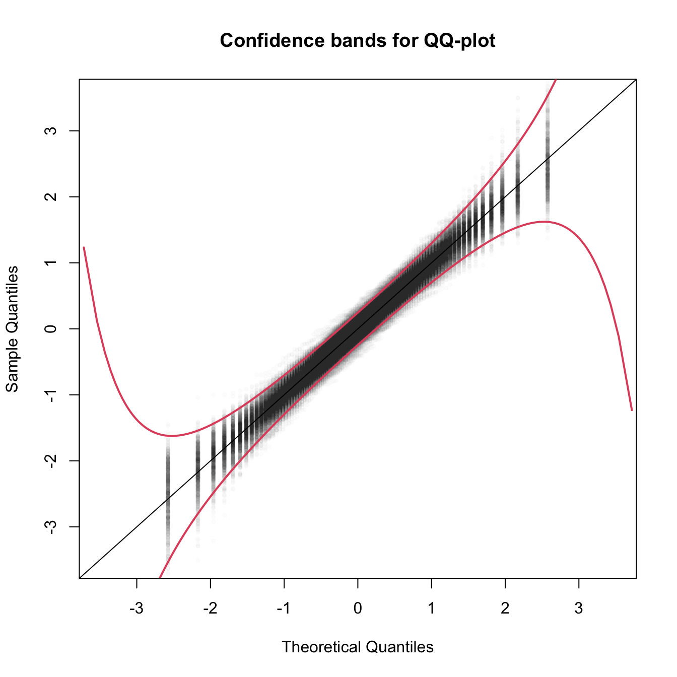

$The uncertainty behind the QQ-plot. The figure aggregates $M=1,000$ different QQ-plots of $\mathcal{N}(0,1)$ data with $n=100,$ displaying for each of them the pairs $(x_p,\hat x_p)$ evaluated at $p=\frac{i-1/2}{n},$ $i=1,\ldots,n$ (as they result from ppoints(n)). The uncertainty is measured by the asymptotic $100(1-\alpha)\%$ CIs for $\hat x_p,$ given by $\left(x_p\pm\frac{z_{\alpha/2}}{\sqrt{n}}\frac{\sqrt{p(1-p)}}{\phi(x_p)}\right).$ These curves are displayed in red for $\alpha=0.05.$ Observe that the vertical strips arise because the $x_p$ coordinate is deterministic.$

Figure 6.5: The uncertainty behind the QQ-plot. The figure aggregates $M=1,000$ different QQ-plots of $\mathcal{N}(0,1)$ data with $n=100,$ displaying for each of them the pairs $(x_p,\hat x_p)$ evaluated at $p=\frac{i-1/2}{n},$ $i=1,\ldots,n$ (as they result from ppoints(n)). The uncertainty is measured by the asymptotic $100(1-\alpha)\%$ CIs for $\hat x_p,$ given by $\left(x_p\pm\frac{z_{\alpha/2}}{\sqrt{n}}\frac{\sqrt{p(1-p)}}{\phi(x_p)}\right).$ These curves are displayed in red for $\alpha=0.05.$ Observe that the vertical strips arise because the $x_p$ coordinate is deterministic.

The Shapiro–Francia test evaluates how tightly distributed the QQ plot is about the linear trend that must arise if the data is normally distributed.

Test purpose. Given $X_1,\ldots,X_n,$ it tests $H_0: F\in\mathcal{F}_\mathcal{N}$ vs. $H_1: F\not\in\mathcal{F}_\mathcal{N}$ consistently against all the alternatives in $H_1.$
Statistic definition and computation. The test statistic, $W_n',$ is simply the squared correlation coefficient for the sample²²⁷

$\begin{align*} \left(\Phi^{-1}\left(\frac{i - 3/8}{n-1/4}\right),X_{(i)}\right),\quad i=1,\ldots,n. \end{align*}$
Distribution under $H_0.$ Royston (1993) derived a simple analytical formula that serves to approximate the null distribution of $W_n'$ for $5\leq n\leq 5,000.$
Highlights and caveats. The test is also parameter-free, since its distribution does not depend on the actual parameters $(\mu,\sigma)$ for which the equality $H_0$ holds.
Implementation in R. The nortest::sf.test function implements the test. The condition $5\leq n\leq 5,000$ is enforced by the function.²²⁸

The use of the function is described below.

# Does not reject H0
set.seed(123456)
n <- 100
x <- rnorm(n = n, mean = 10)
nortest::sf.test(x)
## 
##  Shapiro-Francia normality test
## 
## data:  x
## W = 0.99336, p-value = 0.8401

# Rejects H0
x <- rt(n = n, df = 3)
nortest::sf.test(x)
## 
##  Shapiro-Francia normality test
## 
## data:  x
## W = 0.91545, p-value = 2.754e-05

# Test statistic
cor(x = sort(x), y = qnorm(ppoints(n, a = 3/8)))^2
## [1] 0.9154466

Exercise 6.9 The gamma distribution can be approximated by a normal distribution. Precisely, $\Gamma(\lambda,n)\approx\mathcal{N}\left(\frac{n}{\lambda},\frac{n}{\lambda^2}\right)$ when $n\to\infty.$ The following simulation study is designed to evaluate the accuracy of the approximation with $n\to\infty$ using goodness-of-fit tests. For that purpose, we generate $X_1,\ldots,X_m\sim\Gamma(\lambda,n)$ and run the following tests:

The Kolmogorov–Smirnov, Cramér–von Mises, and Anderson–Darling tests, where $F_0$ stands for the cdf of $\mathcal{N}\left(\frac{n}{\lambda},\frac{n}{\lambda^2}\right).$
The normality adaptations of the previous tests.

Do:

Code a function that simulates $X_1,\ldots,X_m\sim\Gamma(\lambda,n)$ and returns the $p$ -values of the aforementioned tests. The function must take as input $\lambda,$ $n,$ and $m.$ Call this function simulation.
Call the simulation function $M=500$ times for $\lambda=1,$ $n=20,$ and $m=100,$ and represent in a $2\times 3$ plot the histograms of the $p$ -values of the six tests. Comment on the output.
Repeat the experiment for: (i) $n=50,200$ with $m=100;$ and (ii) $m=50,200$ with $n=50.$ Explain the interpretations of the effects of $n$ and $m$ in the results.

6.1.3 Bootstrap-based approach to goodness-of-fit testing

Each normality test discussed in the previous section is an instance of a goodness-of-fit test for a parametric distribution model. Precisely, the normality tests are goodness-of-fit tests for the normal distribution model. Therefore, they address a specific instance of the test of the null composite hypothesis

$\begin{align*} H_0:F\in\mathcal{F}_{\Theta}:=\left\{F_\theta:\theta\in\Theta\subset\mathbb{R}^q\right\}, \end{align*}$

where $\mathcal{F}_{\Theta}$ denotes a certain parametric family of distributions indexed by the (possibly multidimensional) parameter $\theta\in\Theta,$ versus the most general alternative

$\begin{align*} H_1:F\not\in\mathcal{F}_{\Theta}. \end{align*}$

The normality case demonstrated that the goodness-of-fit tests for the simple hypothesis were not readily applicable, and that the null distributions were affected by the estimation of the unknown parameters $\theta=(\mu,\sigma).$ In addition, these null distributions tend to be cumbersome, requiring analytical approximations that have to be done on a test-by-test basis in order to obtain computable $p$ -values.

To make things worse, the derivations that were done to obtain the asymptotic distributions of the normality test are not reusable if $\mathcal{F}_\Theta$ is different. For example, if we wanted to test exponentiality, that is,

$\begin{align} H_0:F\in\mathcal{F}_{\mathbb{R}^+}=\left\{F_\theta(x)=(1-e^{-\theta x})1_{\{x>0\}}:\theta\in\mathbb{R}^+\right\},\tag{6.11} \end{align}$

then new asymptotic distributions with their corresponding new analytical approximations would need to be derived. Clearly, this is not a very practical approach if we are to evaluate the goodness-of-fit of several parametric models. A practical computational-based solution is to rely on bootstrap, specifically, on parametric bootstrap.

Since the main problem is to establish the distribution of the test statistic under $H_0,$ then a possibility is to approximate this distribution by the distribution of the bootstrapped statistic. Precisely, let $T_n$ be the statistic computed from the sample

$\begin{align*} X_1,\ldots,X_n\stackrel{H_0}{\sim}F_\theta \end{align*}$

and let $T_n^*$ be its bootstrapped version, that is, the statistic computed from the simulated sample²²⁹

$\begin{align} X^*_1,\ldots,X^*_n \sim F_{\hat\theta}.\tag{6.12} \end{align}$

Then, if $H_0$ holds, the distribution of $T_n$ is approximated²³⁰ by the one of $T_n^*$ . In addition, since the sampling in (6.12) is completely under our control, we can approximate arbitrarily well the distribution of $T_n^*$ by Monte Carlo. For example, the computation of the upper tail probability $\mathbb{P}^*[T_n^*>x],$ required to obtain $p$ -values in all the tests we have seen, can be done by

$\begin{align*} \mathbb{P}^*[T_n^* > x]\approx\frac{1}{B}\sum_{b=1}^B 1_{\{T_n^{*b}> x\}}, \end{align*}$

where $T_n^{*1},\ldots,T_n^{*B}$ is a sample from $T_n^*$ obtained by simulating $B$ bootstrap samples from (6.12).

The whole approach can be summarized in the following bootstrap-based procedure for performing a goodness-of-fit test for a parametric distribution model:

Estimate $\theta$ from the sample $X_1,\ldots,X_n,$ obtaining $\hat\theta$ (for example, use maximum likelihood).
Compute the statistic $T_n$ from $X_1,\ldots,X_n$ and $\hat\theta.$
Enter the “bootstrap world”. For $b=1,\ldots,B$ :
1. Simulate a boostrap sample $X_1^{*b},\ldots,X_n^{*b}$ from $F_{\hat\theta}.$
2. Compute $\hat\theta^{*b}$ from $X_1^{*b},\ldots,X_n^{*b}$ exactly in the same form that $\hat\theta$ was computed from $X_1,\ldots,X_n.$
3. Compute $T_n^{*b}$ from $X_1^{*b},\ldots,X_n^{*b}$ and $\hat\theta^{*b}.$
Obtain the $p$ -value approximation

$\begin{align*} p\text{-value}\approx\frac{1}{B}\sum_{b=1}^B 1_{\{T_n^{*b}> T_n\}} \end{align*}$

and emit a test decision from it. Modify it accordingly if rejection of $H_0$ does not happen for large values of $T_n.$

The following chunk of code provides a template function for implementing the previous algorithm. The template is initialized with the specifics for testing (6.11), for which $\hat\theta_{\mathrm{ML}}=1/{\bar X}.$ The function uses the boot::boot function for carrying out the parametric bootstrap.

# A goodness-of-fit test of the exponential distribution using the
# Cramér-von Mises statistic
cvm_exp_gof <- function(x, B = 5e3, plot_boot = TRUE) {

  # Test statistic function (depends on the data only)
  Tn <- function(data) {

    # Maximum likelihood estimator -- MODIFY DEPENDING ON THE PROBLEM
    theta_hat <- 1 / mean(data)

    # Test statistic -- MODIFY DEPENDING ON THE PROBLEM
    goftest::cvm.test(x = data, null = "pexp", rate = theta_hat)$statistic

  }

  # Function to simulate bootstrap samples X_1^*, ..., X_n^*. Requires TWO
  # arguments, one being the data X_1, ..., X_n and the other containing
  # the parameter theta
  r_mod <- function(data, theta) {

    # Simulate from an exponential. In this case, the function only uses
    # the sample size from the data argument to estimate theta -- MODIFY
    # DEPENDING ON THE PROBLEM
    rexp(n = length(data), rate = 1 / theta)

  }

  # Estimate of theta -- MODIFY DEPENDING ON THE PROBLEM
  theta_hat <- 1 / mean(x)

  # Perform bootstrap resampling with the aid of boot::boot
  Tn_star <- boot::boot(data = x, statistic = Tn, sim = "parametric", 
                        ran.gen = r_mod, mle = theta_hat, R = B)

  # Test information -- MODIFY DEPENDING ON THE PROBLEM
  method <- "Bootstrap-based Cramér-von Mises test for exponentiality"
  alternative <- "any alternative to exponentiality"

  # p-value: modify if rejection does not happen for large values of the
  # test statistic. $t0 is the original statistic and $t has the bootstrapped
  # ones.
  pvalue <- mean(Tn_star$t > Tn_star$t0)

  # Construct an "htest" result
  result <- list(statistic = c("stat" = Tn_star$t0), p.value = pvalue,
                 theta_hat = theta_hat, statistic_boot = drop(Tn_star$t),
                 B = B, alternative = alternative, method = method,
                 data.name = deparse(substitute(x)))
  class(result) <- "htest"

  # Plot the position of the original statistic with respect to the
  # bootstrap replicates?
  if (plot_boot) {

    hist(result$statistic_boot, probability = TRUE, 
         main = paste("p-value:", result$p.value), 
         xlab = latex2exp::TeX("$T_n^*$"))
    rug(result$statistic_boot)
    abline(v = result$statistic, col = 2, lwd = 2)
    text(x = result$statistic, y = 1.5 * mean(par()$usr[3:4]),
         labels = latex2exp::TeX("$T_n$"), col = 2, pos = 4)

  }

  # Return "htest"
  return(result)

}

# Check the test for H0 true
set.seed(123456)
x <- rgamma(n = 100, shape = 1, scale = 1)
gof0 <- cvm_exp_gof(x = x, B = 1e3)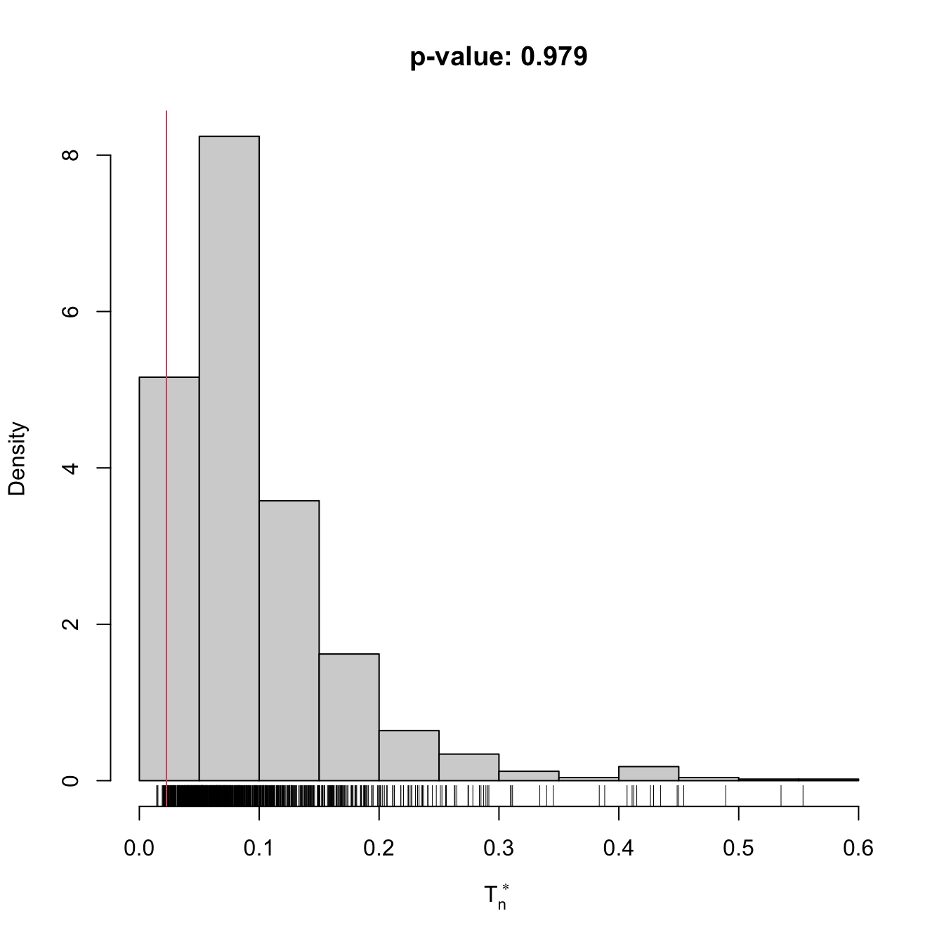

gof0
## 
##  Bootstrap-based Cramér-von Mises test for exponentiality
## 
## data:  x
## stat.omega2 = 0.022601, p-value = 0.979
## alternative hypothesis: any alternative to exponentiality

# Check the test for H0 false
x <- rgamma(n = 100, shape = 2, scale = 1)
gof1 <- cvm_exp_gof(x = x, B = 1e3)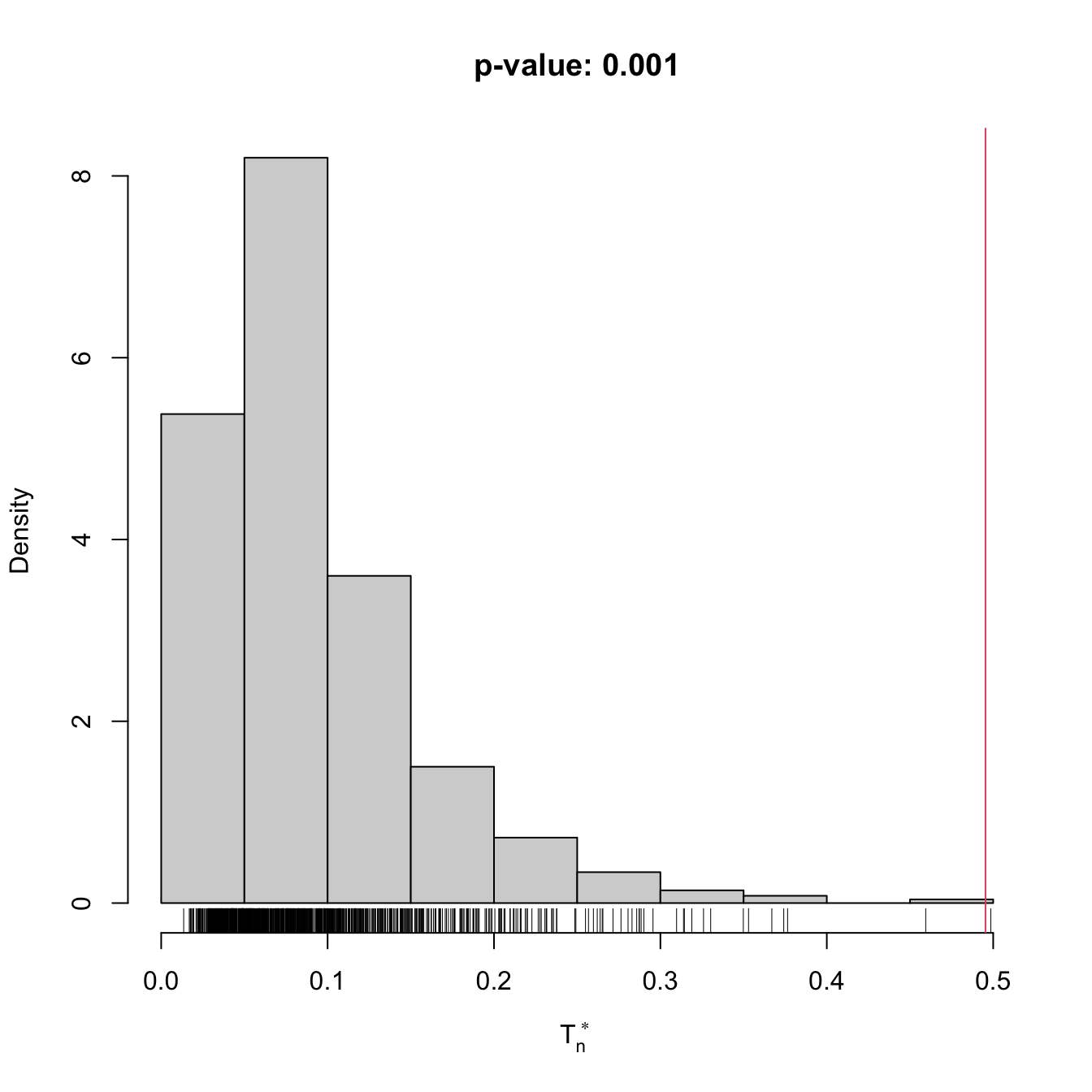

gof1
## 
##  Bootstrap-based Cramér-von Mises test for exponentiality
## 
## data:  x
## stat.omega2 = 0.49536, p-value = 0.001
## alternative hypothesis: any alternative to exponentiality

Another example is given below. It adapts the previous template for the flexible class of mixtures of normal distributions given in (2.32).

# A goodness-of-fit test of a mixture of m normals using the
# Cramér-von Mises statistic
cvm_nm_gof <- function(x, m, B = 1e3, plot_boot = TRUE) {

  # Test statistic function (depends on the data only)
  Tn <- function(data) {

    # EM algorithm for fitting normal mixtures. With trace = 0 we disable the
    # default convergence messages or otherwise they will saturate the screen
    # with the bootstrap loop. Be aware that this is a potentially dangerous
    # practice, as we may lose important information about the convergence of
    # the EM algorithm
    theta_hat <- nor1mix::norMixEM(x = data, m = m, trace = 0)

    # Test statistic
    goftest::cvm.test(x = data, null = nor1mix::pnorMix, 
                      obj = theta_hat)$statistic

  }

  # Function to simulate bootstrap samples X_1^*, ..., X_n^*. Requires TWO
  # arguments, one being the data X_1, ..., X_n and the other containing
  # the parameter theta
  r_mod <- function(data, theta) {

    nor1mix::rnorMix(n = length(data), obj = theta)

  }

  # Estimate of theta
  theta_hat <- nor1mix::norMixEM(x = x, m = m, trace = 0)

  # Perform bootstrap resampling with the aid of boot::boot
  Tn_star <- boot::boot(data = x, statistic = Tn, sim = "parametric", 
                        ran.gen = r_mod, mle = theta_hat, R = B)

  # Test information
  method <- "Bootstrap-based Cramér-von Mises test for normal mixtures"
  alternative <- paste("any alternative to a", m, "normal mixture")

  # p-value: modify if rejection does not happen for large values of the
  # test statistic. $t0 is the original statistic and $t has the bootstrapped
  # ones.
  pvalue <- mean(Tn_star$t > Tn_star$t0)

  # Construct an "htest" result
  result <- list(statistic = c("stat" = Tn_star$t0), p.value = pvalue,
                 theta_hat = theta_hat, statistic_boot = drop(Tn_star$t),
                 B = B, alternative = alternative, method = method,
                 data.name = deparse(substitute(x)))
  class(result) <- "htest"

  # Plot the position of the original statistic with respect to the
  # bootstrap replicates?
  if (plot_boot) {

    hist(result$statistic_boot, probability = TRUE, 
         main = paste("p-value:", result$p.value), 
         xlab = latex2exp::TeX("$T_n^*$"))
    rug(result$statistic_boot)
    abline(v = result$statistic, col = 2, lwd = 2)
    text(x = result$statistic, y = 1.5 * mean(par()$usr[3:4]),
         labels = latex2exp::TeX("$T_n$"), col = 2, pos = 4)

  }

  # Return "htest"
  return(result)

}

# Check the test for H0 true
set.seed(123456)
x <- c(rnorm(n = 100, mean = 2, sd = 0.5), rnorm(n = 100, mean = -2))
gof0 <- cvm_nm_gof(x = x, m = 2, B = 1e3)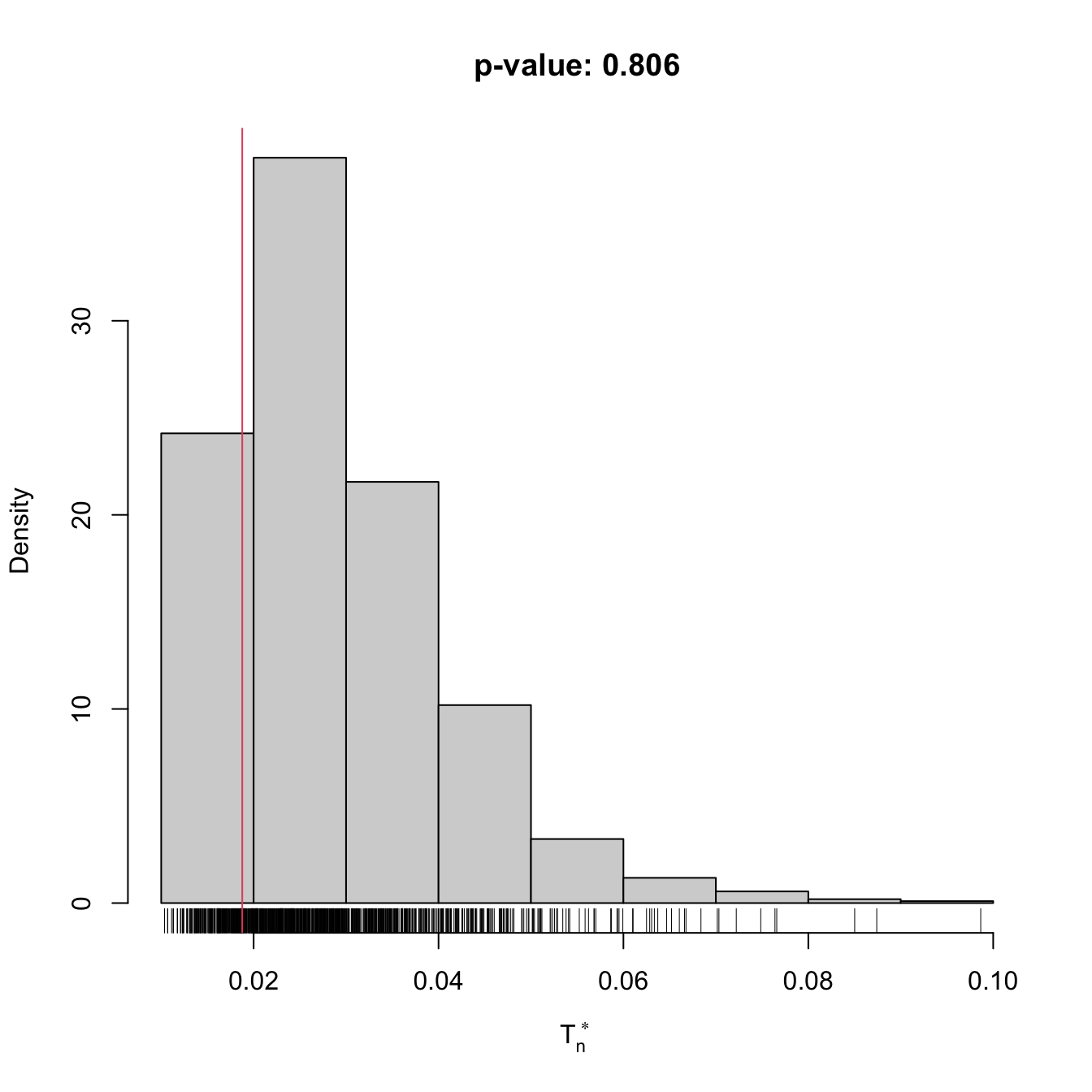

gof0
## 
##  Bootstrap-based Cramér-von Mises test for normal mixtures
## 
## data:  x
## stat.omega2 = 0.018769, p-value = 0.806
## alternative hypothesis: any alternative to a 2 normal mixture

# Graphical assessment that H0 (parametric fit) and data (kde) match
plot(gof0$theta_hat, p.norm = FALSE, ylim = c(0, 0.5))
plot(ks::kde(x), col = 2, add = TRUE)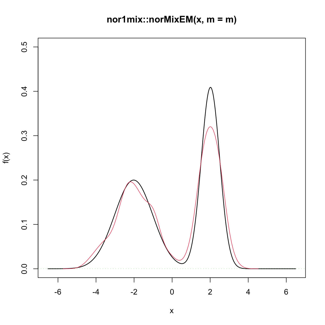


# Check the test for H0 false
x <- rgamma(n = 100, shape = 2, scale = 1)
gof1 <- cvm_nm_gof(x = x, m = 1, B = 1e3)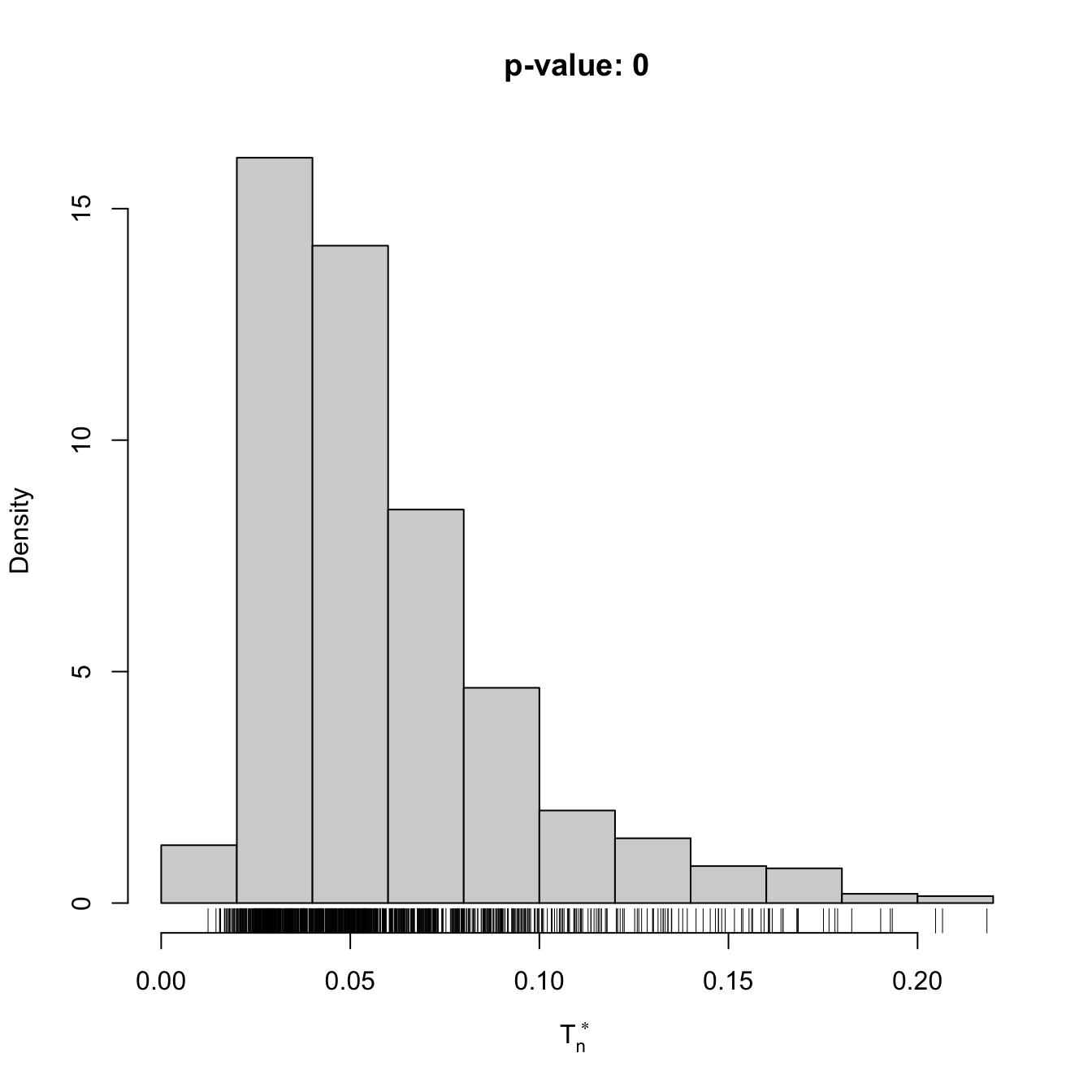

gof1
## 
##  Bootstrap-based Cramér-von Mises test for normal mixtures
## 
## data:  x
## stat.omega2 = 0.44954, p-value < 2.2e-16
## alternative hypothesis: any alternative to a 1 normal mixture

# Graphical assessment that H0 (parametric fit) and data (kde) do not match
plot(gof1$theta_hat, p.norm = FALSE, ylim = c(0, 0.5))
plot(ks::kde(x), col = 2, add = TRUE)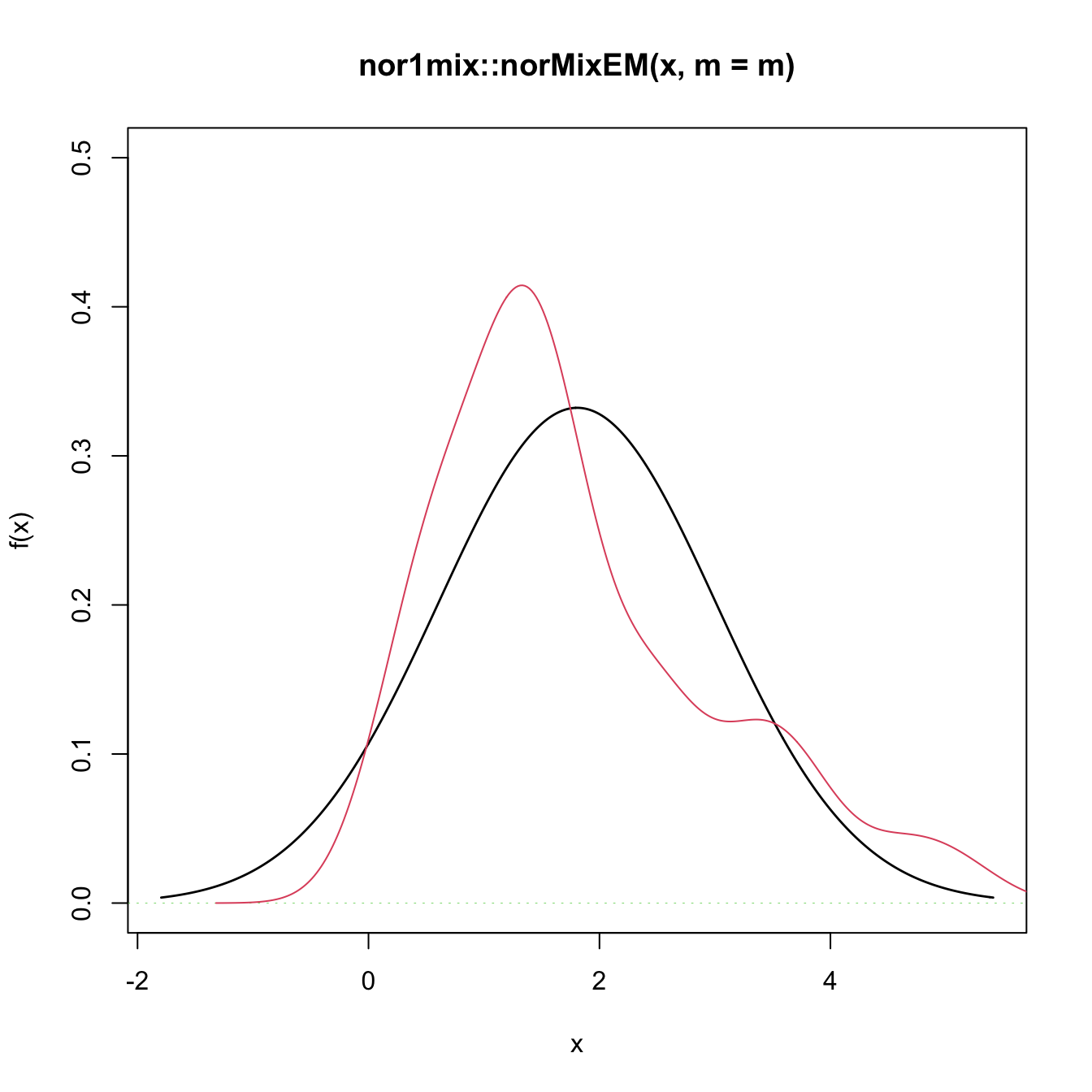

Exercise 6.10 Change in the previous example the number of mixture components to $m=3$ and $m=10,$ using the same sample as in the example. Do you reject the null hypothesis? Why? What about $m=1$ ? Try with new simulated datasets.

Exercise 6.11 Adapt the previous template to perform the following tasks:

Test the goodness-of-fit of the Weibull distribution using the Anderson–Darling statistic. Check with a small simulation study that the test is correctly implemented (such that the significance level $\alpha$ is respected if $H_0$ holds).
Test the goodness-of-fit of the lognormal distribution using the Anderson–Darling statistic. Check with a small simulation study that the test is correctly implemented.
Apply the previous two tests to inspect if av_gray_one from Exercise 2.25 and if temps-other.txt are distributed according to a Weibull or lognormal. Explain the results.

References

Barrio, E. del. 2007. “Empirical and Quantile Processes in the Asymptotic Theory of Goodness-of-Fit Tests.” In Lectures on Empirical Processes, 1–92. EMS Series of Lectures in Mathematics. Zürich: European Mathematical Society. https://doi.org/10.4171/027.

D’Agostino, R. B., and M. A. Stephens, eds. 1986. Goodness-of-Fit Techniques. Vol. 68. Statistics: Textbooks and Monographs. New York: Marcel Dekker. https://www.routledge.com/Goodness-of-Fit-Techniques/DAgostino/p/book/9780367580346.

Dallal, G. E., and L. Wilkinson. 1986. “An Analytic Approximation to the Distribution of Lilliefors’s Test Statistic for Normality.” The American Statistician 40 (4): 294–96. https://doi.org/10.1080/00031305.1986.10475419.

Lilliefors, H. W. 1967. “On the Kolmogorov-Smirnov Test for Normality with Mean and Variance Unknown.” Journal of the American Statistical Association 62 (318): 399–402. https://doi.org/10.1080/01621459.1967.10482916.

Royston, P. 1993. “A Pocket-Calculator Algorithm for the Shapiro-Francia Test for Non-Normality: An Application to Medicine.” Statistics in Medicine 12 (2): 181–84. https://doi.org/10.1002/sim.4780120209.

Shao, J. 1999. Mathematical Statistics. Springer Texts in Statistics. New York: Springer. https://doi.org/10.1007/b97553.

Stephens, M. A. 1974. “EDF Statistics for Goodness of Fit and Some Comparisons.” Journal of the American Statistical Association 69 (347): 730–37. https://doi.org/10.2307/2286009.

$F$ does not need to be continuous.↩︎
The fact that $F=F_0$ is tested in full generality against any distribution that is different from $F_0$ raises the omnibus test (all-purpose test) terminology for the kind of tests that are able to detect all the alternatives to $H_0$ that are within $H_1.$ ↩︎
That is, the tests will have a rejection probability lower than $\alpha$ when $H_0$ is true.↩︎
If $F$ and $F_0$ were continuous, the density approach to this problem would compare the kde $\hat{f}(\cdot;h)$ seen in Chapter 2 with the density $f_0.$ While using a kde for testing $H_0:F=F_0$ via $H_0:f=f_0$ is a perfectly valid approach and has certain advantages (e.g., better detection of local violations of $H_0$ ), it is also more demanding (it requires selecting the bandwidth $h$ ) and limited (applicable to continuous random variables only). The cdf optic, although not appropriate for visualization or for the applications described in Section 3.5, suffices for conducting hypothesis testing in a nonparametric way.↩︎
A popular approach to goodness-of-fit tests, not covered in these notes, is the chi-squared test (see ?chisq.test). This test is based on aggregating the values of $X$ in $k$ classes $I_i,$ $i=1,\ldots,k,$ where $\cup_{i=1}^k I_i$ cover the support of $X.$ Worryingly, one can modify the outcome of the test by altering the form of these classes and the choice of $k$ – a sort of tuning parameter. The choice of $k$ also affects the quality of the asymptotic null distribution. Therefore, for continuous and discrete random variables, the chi-squared test has significant drawbacks when compared to the ecdf-based tests. Nevertheless, the “chi-squared philosophy” of testing is remarkably general: as opposed to ecdf-based tests, it can be readily applied to the analysis of categorical variables and contingency tables.↩︎
Or the $\infty$ -distance $\|F_n-F_0\|_\infty=\sup_{x\in\mathbb{R}} \left|F_n(x)-F_0(x)\right|.$ ↩︎
With the addition of the $\sqrt{n}$ factor in order to standardize $D_n$ in terms of its asymptotic distribution under $H_0.$ Many authors do not consider this factor as a part of the test statistic itself.↩︎
Notice that $F_n(X_{(i)})=\frac{i}{n}$ and $F_n(X_{(i)}^-)=\frac{i-1}{n}.$ ↩︎
When the sample size $n$ is large: $n\to\infty.$ ↩︎
The infinite series converges quite fast and $50$ terms are usually enough to evaluate (6.3) with high accuracy for $x\in\mathbb{R}.$ ↩︎
A tie occurs when two elements of the sample are numerically equal, an event with probability zero if the sample comes from a truly continuous random variable.↩︎
More precisely, the pdf of $D_n$ would follow from the joint pdf of the sorted sample $(U_{(1)},\ldots,U_{(n)})$ that is generated from a $\mathcal{U}(0,1)$ and for which the transformation (6.2) is employed. The exact analytical formula, for a given $n,$ is very cumbersome, hence the need for an asymptotic approximation.↩︎
That is, if $F_0$ is the cdf of a $\mathcal{N}(0,1)$ or the cdf of a $\mathrm{Exp}(\lambda),$ the distribution of $D_n$ under $H_0$ is exactly the same.↩︎
Ties may appear as a consequence of a measuring process of a continuous quantity having low precision.↩︎
Which is $\lim_{n\to\infty}\mathbb{P}[d_n>D_n]=1-K(d_n),$ where $d_n$ is the observed statistic and $D_n$ is the random variable (6.2).↩︎
Recall that the $p$ -value of any statistical test is a random variable, since it depends on the sample.↩︎
Recall that $\mathrm{d}F_0(x)=f_0(x)\,\mathrm{d}x$ if $F_0$ is continuous.↩︎
See page 10 in Barrio (2007).↩︎
See, e.g., Section 5 in Stephens (1974) or page 110 in D’Agostino and Stephens (1986). Observe this is only empirical evidence for certain scenarios.↩︎
The motivation for considering $w(x)=(F_0(x)(1-F_0(x)))^{-1}$ stems from recalling that $\mathbb{E}[(F_n(x)-F_0(x))^2]\stackrel{H_0}{=}F_0(x)(1-F_0(x))/n$ (see Example 1.8). That is, estimating $F_0$ on the tails is less variable than at its center. $A_n^2$ weights $(F_n(x)-F_0(x))^2$ with its variability by incorporating $w.$ ↩︎
Actually, due to the allocation of greater weight to the tails, the statistic $A_n^2$ is somehow on the edge of existence. If $F_0$ is continuous, the weight function $w(x)=(F_0(x)(1-F_0(x)))^{-1}$ is not integrable on $\mathbb{R}.$ Indeed, $\int w(x)\,\mathrm{d}F_0(x)=\int_0^1 (x(1-x))^{-1}\,\mathrm{d}x=\nexists.$ It is only thanks to the factor $(F_n(x)-F_0(x))^2$ in the integrand that $A_n^2$ is well defined.↩︎
Importantly, recall that $P_1,\ldots,P_n$ are not independent, since $\bar{X}$ and $\hat{S}$ depend on the whole sample $X_1,\ldots,X_n.$ To dramatize this point, imagine that $X_1$ is very large. Then, it would drive $\frac{X_i-\bar{X}}{\hat{S}}$ towards large negative values, revealing the dependence of $P_2,\ldots,P_n$ on $P_1.$ This is a very remarkable qualitative difference with respect to $U_1,\ldots,U_n,$ which was an iid sample. $P_1,\ldots,P_n$ is an id sample, but not an iid sample.↩︎
$H_0$ is rejected with significance level $\alpha$ if the statistic is above the critical value for $\alpha.$ ↩︎
The precise form of $\tilde{f}_0$ (if $S$ stands for the quasi-variance) can be seen in equation (3.1) in Shao (1999).↩︎
The Shapiro–Wilk test is implemented in the shapiro.test R function. The test has the same highlights and caveats as nortest::sf.test.↩︎
Minor modifications of the $\frac{i}{n+1}$ -lower quantile $\Phi^{-1}\left(\frac{i}{n+1}\right)$ may be considered.↩︎
For $X\sim F,$ the $p$ -th quantile $x_p=F^{-1}(p)$ of $X$ is estimated through the sample quantile $\hat{x}_p:=F_n^{-1}(p).$ If $X\sim f$ is continuous, then $\sqrt{n}(\hat{x}_p-x_p)$ is asymptotically $\mathcal{N}\left(0,\frac{p(1-p)}{f(x_p)^2}\right).$ Therefore, the variance of $\hat x_p$ grows if $p\to0,1$ and more variability is expected in the extremes of the QQ-plot.↩︎
Observe that qnorm(ppoints(x, a = 3 / 8)) is used as an approximation to the expected ordered quantiles from a $\mathcal{N}(0,1),$ whereas qnorm(ppoints(x, a = 1 / 2)) is employed internally in qqplot.↩︎
However, the R code of the function allows computing the statistic and carrying out a bootstrap-based test as described in Section 6.1.3 for $n\geq5,000.$ The shapiro.test function, on the contrary, does not allow this simple extraction, as the core of the function is written in C (function C_SWilk) and internally enforces the condition $5\leq n\leq 5,000.$ ↩︎
Notice that $X^*_i$ is always distributed as $F_{\hat\theta},$ no matter whether $H_0$ holds or not.↩︎
With increasing precision as $n\to\infty.$ ↩︎