Chapter 3 Kernel density estimation II

Like in the univariate case, any random vector $\mathbf{X}$ supported in $\mathbb{R}^p$ is completely characterized by its cdf. However, cdfs are even harder to visualize and interpret when $p>1,$ as the accumulation of probability happens simultaneously in several directions. As a consequence, densities become highly valuable tools for data exploration, especially for dimensions $p=2,3.$

Densities characterize continuous random vectors $\mathbf{X}$ and are key building blocks for a variety of highly successful multivariate methods. Indeed, many of them may be seen as connected to the omnipresent normal distribution.

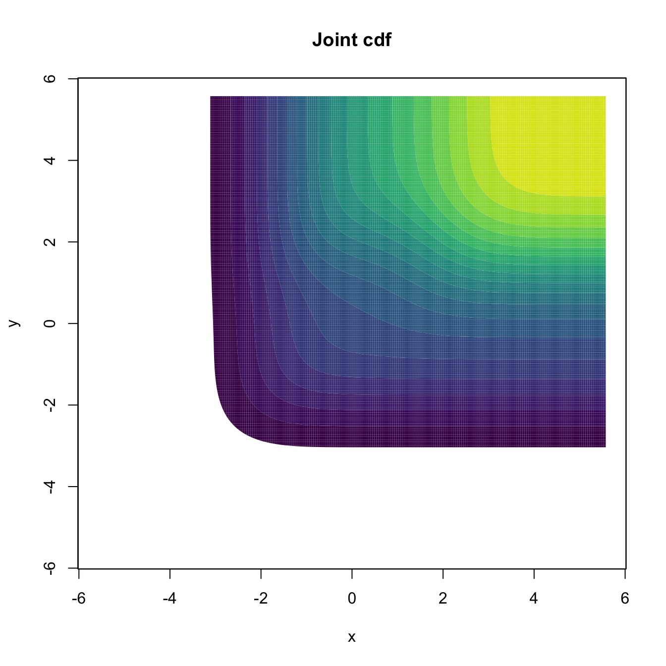
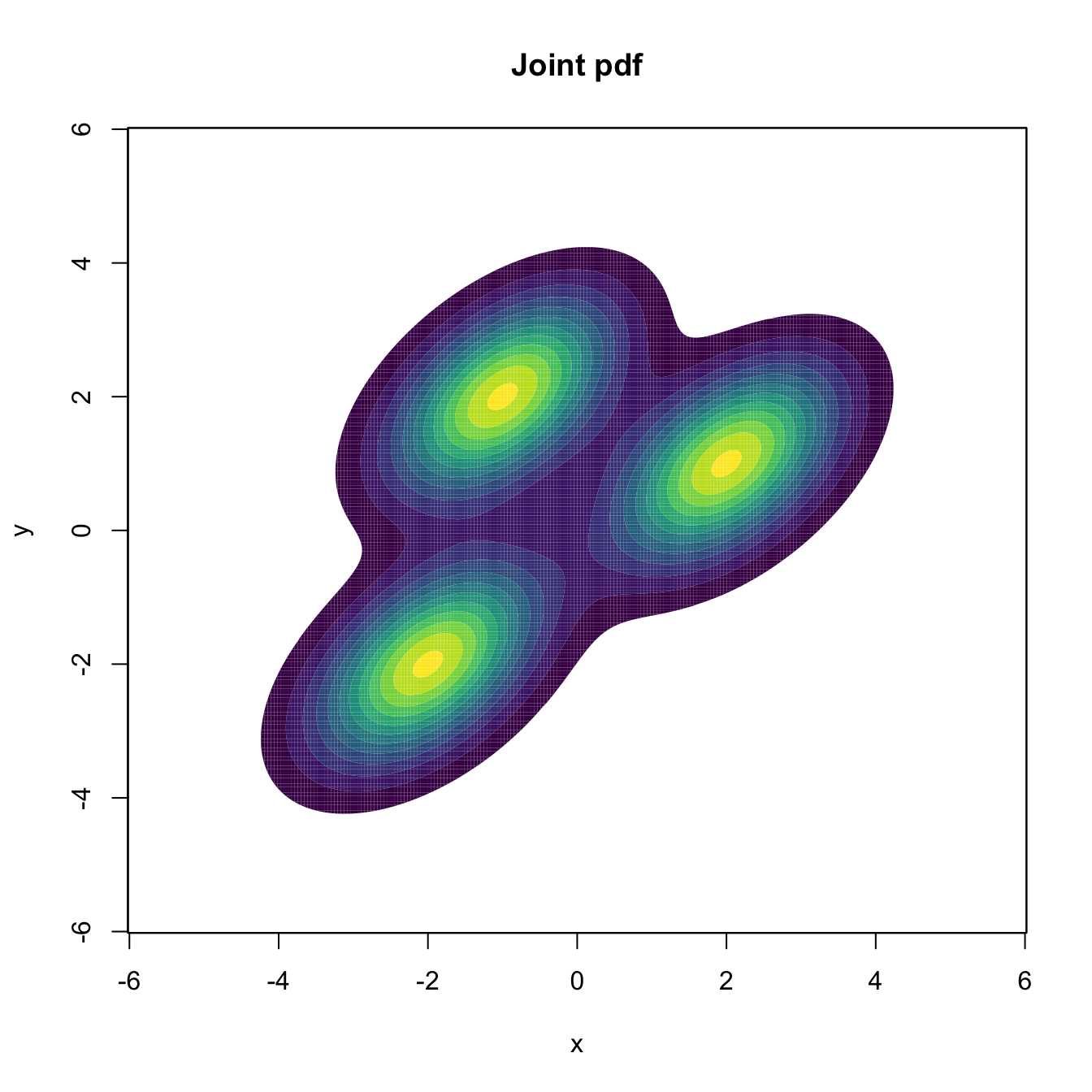
$The contour levels of the joint cdf and pdf for a mixture of three bivariate normals. Clearly, the pdf surface yields insights into the structure of the continuous random vector $\mathbf{X},$ whereas the cdf gives hardly any.$ $The contour levels of the joint cdf and pdf for a mixture of three bivariate normals. Clearly, the pdf surface yields insights into the structure of the continuous random vector $\mathbf{X},$ whereas the cdf gives hardly any.$

Figure 3.1: The contour levels of the joint cdf and pdf for a mixture of three bivariate normals. Clearly, the pdf surface yields insights into the structure of the continuous random vector $\mathbf{X},$ whereas the cdf gives hardly any.

As we will see in this chapter, the concepts associated with multivariate density estimation extend quite straightforwardly from the univariate situation. However, despite this conceptual simplicity, and as often happens with any problem in statistics, density estimation in $\mathbb{R}^p$ becomes more and more complex as the dimension $p$ increases.