5.3 Prediction and confidence intervals
Prediction via the conditional expectation \(m(\mathbf{x})=\mathbb{E}[Y|\mathbf{X}=\mathbf{x}]\) reduces to evaluate \(\hat{m}(\mathbf{x};q,\mathbf{h}).\) The fitted values are, therefore, \(\hat{Y}_i:=\hat{m}(\mathbf{X}_i;q,\mathbf{h}),\) \(i=1,\ldots,n.\) The np package has methods to perform these operations via the predict and fitted functions.
More interesting is the discussion about the uncertainty of \(\hat{m}(\mathbf{x};q,\mathbf{h})\) and, as a consequence, of the predictions. Differently to what happened in parametric models, in nonparametric regression there is no parametric distribution of the response that can help to carry out the inference and, consequently, to address the uncertainty of the estimation. Because of this: (i) the prediction interest is mainly focused on the conditional expectation \(m(\mathbf{x})=\mathbb{E}[Y|\mathbf{X}=\mathbf{x}]\) and not on the conditional response \(Y|\mathbf{X}=\mathbf{x}\); and (ii) it is required to resort to somewhat convoluted asymptotic expressions184 that rely on plugging-in estimates for the unknown terms on the asymptotic bias and variance. The next code chunk exemplifies how to compute asymptotic confidence intervals with np, both for the marginal effects and the conditional expectation \(m(\mathbf{x}).\) In the latter case, the confidence intervals are \((\hat{m}(\mathbf{x};q,\mathbf{h})\pm z_{\alpha/2}\hat{\mathrm{se}}(\hat{m}(\mathbf{x};q,\mathbf{h}))),\) where \(\hat{\mathrm{se}}(\hat{m}(\mathbf{x};q,\mathbf{h}))\) is the asymptotic estimation of the standard deviation of \(\hat{m}(\mathbf{x};q,\mathbf{h}).\)
# Asymptotic confidence bands for the marginal effects of each predictor on
# the response
par(mfrow = c(2, 3))
plot(fit_OECD, plot.errors.method = "asymptotic", common.scale = FALSE,
     plot.par.mfrow = FALSE, col = 2)
# The asymptotic standard errors associated with the regression evaluated at
# the evaluation points are in $merr
head(fit_OECD$merr)
## [1] 0.007982761 0.006815515 0.002888752 0.002432522 0.005004411 0.008483572

# Recall that in $mean we had the regression evaluated at the evaluation points,
# by default the sample of the predictors, so in this case it is the same as
# the fitted values
head(fit_OECD$mean)
## [1] 0.02213477 0.02460647 0.03216185 0.04167737 0.01068088 0.04456299

# Fitted values
head(fitted(fit_OECD))
## [1] 0.02213477 0.02460647 0.03216185 0.04167737 0.01068088 0.04456299

# Prediction for the first 3 points + asymptotic standard errors
pred <- predict(fit_OECD, newdata = oecdpanel[1:3, ], se.fit = TRUE)

# Predictions
pred$fit
## [1] 0.02213477 0.02460647 0.03216185

# Manual computation of the asymptotic 100 * (1 - alpha)% confidence intervals
# for the conditional mean of the first 3 points
alpha <- 0.05
z_alpha2 <- qnorm(1 - alpha / 2)
cbind(pred$fit - z_alpha2 * pred$se.fit, pred$fit + z_alpha2 * pred$se.fit)
##            [,1]       [,2]
## [1,] 0.00648885 0.03778070
## [2,] 0.01124831 0.03796464
## [3,] 0.02649999 0.03782370

# Recall that z_alpha2 is almost 2
z_alpha2
## [1] 1.959964
A non-asymptotic alternative to approximate the sampling distribution of \(\hat{m}(\mathbf{x};q,\mathbf{h})\) is a bootstrap resampling procedure. Indeed, bootstrap approximations of confidence intervals for \(m(\mathbf{x}),\) if performed adequately, are generally more trustworthy than asymptotic approximations.185 Naive bootstrap resampling is np’s default bootstrap procedure to compute confidence intervals for \(m(\mathbf{x})\) using the estimator \(\hat{m}(\mathbf{x};q,\mathbf{h}).\) This procedure is summarized as follows:
- Compute \(\hat{m}(\mathbf{x};q,\mathbf{h})=\sum_{i=1}^n W_i^q(\mathbf{x})Y_i\) from the original sample \((\mathbf{X}_1,Y_1),\ldots,(\mathbf{X}_n,Y_n).\)
- Enter the “bootstrap world”. For \(b=1,\ldots,B\):
- Obtain the bootstrap sample \((\mathbf{X}_1^{*b},Y_1^{*b}),\ldots,(\mathbf{X}_n^{*b},Y_n^{*b})\) by drawing, with replacement, random observations from the set \(\{(\mathbf{X}_1,Y_1),\ldots, (\mathbf{X}_n,Y_n)\}.\)186
- Compute \(\hat{m}^{*b}(\mathbf{x};q,\mathbf{h})=\sum_{i=1}^n W_i^{q,\,*b}(\mathbf{x})Y_i^{*b}\) from \((\mathbf{X}_1^{*b},Y_1^{*b}),\ldots,\) \((\mathbf{X}_n^{*b},Y_n^{*b}).\)
- From \(\hat{m}(\mathbf{x};q,\mathbf{h})\) and \(\{\hat{m}^{*b}(\mathbf{x};q,\mathbf{h})\}_{b=1}^B,\) compute a bootstrap \(100(1-\alpha)\%\)-confidence interval for \(m(\mathbf{x}).\) The two most common approaches for doing so are:
- Normal approximation (
"standard"): \(\big(\hat{m}(\mathbf{x};q,\mathbf{h})\pm z_{\alpha/2}\hat{\mathrm{se}}^*(\hat{m}(\mathbf{x};q,\mathbf{h}))\big),\) where \(\hat{\mathrm{se}}^*(\hat{m}(\mathbf{x};q,\mathbf{h}))\) is the sample standard deviation of \(\{\hat{m}^{*b}(\mathbf{x};q,\mathbf{h})\}_{b=1}^B.\) - Quantile-based (
"quantile"): \(\big(m_{\alpha/2}^*,m_{1-\alpha/2}^*\big),\) where \(m_{\alpha}^*\) is the (lower) sample \(\alpha\)-quantile of \(\{\hat{m}^{*b}(\mathbf{x};q,\mathbf{h})\}_{b=1}^B.\)
- Normal approximation (
Bootstrap standard errors are entirely computed by np::npplot (and neither by np::npreg nor predict, as for asymptotic standard errors). The default method, plot.errors.boot.method = "inid", implements the naive bootstrap to approximate the confidence intervals of the marginal effects.187
# Bootstrap confidence bands (using naive bootstrap, the default)
# They take more time to compute because a resampling + refitting takes place
B <- 200
par(mfrow = c(2, 3))
plot(fit_OECD, plot.errors.method = "bootstrap", common.scale = FALSE,
     plot.par.mfrow = FALSE, plot.errors.boot.num = B, random.seed = 42,
     col = 2)
# plot.errors.boot.num is B and defaults to 399
# random.seed fixes the seed to always get the same bootstrap errors. It
# defaults to 42 if not specified
The following chunk of code helps extracting the information about the bootstrap confidence intervals from the call to np::npplot and illustrates further bootstrap options.
# Univariate local constant regression with CV bandwidth
bw1 <- np::npregbw(formula = growth ~ initgdp, data = oecdpanel, regtype = "lc")
fit1 <- np::npreg(bw1)
summary(fit1)
##
## Regression Data: 616 training points, in 1 variable(s)
##                 initgdp
## Bandwidth(s): 0.2774471
##
## Kernel Regression Estimator: Local-Constant
## Bandwidth Type: Fixed
## Residual standard error: 0.02907224
## R-squared: 0.08275453
##
## Continuous Kernel Type: Second-Order Gaussian
## No. Continuous Explanatory Vars.: 1

# Asymptotic (not bootstrap) standard errors
head(fit1$merr)
## [1] 0.002229093 0.002342670 0.001712938 0.002210457 0.002390530 0.002333956

# Normal approximation confidence intervals with plot.errors.type = "standard"
# (default) + extraction of errors with plot.behavior = "plot-data"
npplot_std <- plot(fit1, plot.errors.method = "bootstrap",
                   plot.errors.type = "standard", plot.errors.boot.num = B,
                   plot.errors.style = "bar", plot.behavior = "plot-data",
                   lwd = 2)
lines(npplot_std$r1$eval[, 1], npplot_std$r1$mean + npplot_std$r1$merr[, 1],
      col = 2, lty = 2)
lines(npplot_std$r1$eval[, 1], npplot_std$r1$mean + npplot_std$r1$merr[, 2],
      col = 2, lty = 2)
# These bootstrap standard errors are different from the asymptotic ones
head(npplot_std$r1$merr)
##              [,1]        [,2]
## [1,] -0.017509208 0.017509208
## [2,] -0.015174698 0.015174698
## [3,] -0.012930989 0.012930989
## [4,] -0.010925377 0.010925377
## [5,] -0.009276906 0.009276906
## [6,] -0.008031584 0.008031584

# Quantile confidence intervals + extraction of errors
npplot_qua <- plot(fit1, plot.errors.method = "bootstrap",
                   plot.errors.type = "quantiles", plot.errors.boot.num = B,
                   plot.errors.style = "bar", plot.behavior = "plot-data")
lines(npplot_qua$r1$eval[, 1], npplot_qua$r1$mean + npplot_qua$r1$merr[, 1],
      col = 2, lty = 2)
lines(npplot_qua$r1$eval[, 1], npplot_qua$r1$mean + npplot_qua$r1$merr[, 2],
      col = 2, lty = 2)
# These bootstrap standard errors are different from the asymptotic ones,
# and also from the previous bootstrap errors (different confidence
# interval method)
head(npplot_qua$r1$merr)
##              [,1]        [,2]
## [1,] -0.016923716 0.017015321
## [2,] -0.015649920 0.015060896
## [3,] -0.012913035 0.012441999
## [4,] -0.010752339 0.009864879
## [5,] -0.008496998 0.008547620
## [6,] -0.006912847 0.007220871
There is no predict() method featuring bootstrap confidence intervals, it has to be coded manually! This is the purpose of the next function, np_pred_CI(), which implements the naive bootstrap procedure described above to compute bootstrap confidence intervals for \(m(\mathbf{x}).\)
# Function to predict and compute bootstrap confidence intervals for m(x). Takes
# as main arguments a np::npreg object (npfit) and the values of the predictors
# where to carry out prediction (exdat). Requires that exdat is a data.frame of
# the same type than the one used for the predictors (e.g., there will be an
# error if one variable appears as a factor for computing npfit and then is
# passed as a numeric in exdat)
np_pred_CI <- function(npfit, exdat, B = 200, conf = 0.95,
                       type_CI = c("standard", "quantiles")[1]) {

  # Extract predictors
  xdat <- npfit$eval

  # Extract response, using a trick from np::npplot.rbandwidth
  tt <- terms(npfit$bws)
  tmf <- npfit$bws$call[c(1, match(c("formula", "data"),
                                   names(npfit$bws$call)))]
  tmf[[1]] <- as.name("model.frame")
  tmf[["formula"]] <- tt
  tmf <- eval(tmf, envir = environment(tt))
  ydat <- model.response(tmf)

  # Predictions
  m_hat <- np::npreg(txdat = xdat, tydat = ydat, exdat = exdat,
                     bws = npfit$bws)$mean

  # Function for performing Step 3
  boot_function <- function(data, indices) {

    np::npreg(txdat = xdat[indices,], tydat = ydat[indices],
              exdat = exdat, bws = npfit$bws)$mean

  }

  # Carry out Step 3
  m_hat_star <- boot::boot(data = data.frame(xdat), statistic = boot_function,
                           R = B)$t

  # Confidence intervals
  alpha <- 1 - conf
  if (type_CI == "standard") {

    z <- qnorm(p = 1 - alpha / 2)
    se <- apply(m_hat_star, 2, sd)
    lwr <- m_hat - z * se
    upr <- m_hat + z * se

  } else if (type_CI == "quantiles") {

    q <- apply(m_hat_star, 2, quantile, probs = c(alpha / 2, 1 - alpha / 2))
    lwr <- q[1, ]
    upr <- q[2, ]

  } else {

    stop("Incorrect type_CI")

  }

  # Return evaluation points, estimates, and confidence intervals
  return(data.frame("exdat" = exdat, "m_hat" = m_hat, "lwr" = lwr, "upr" = upr))

}

# Obtain predictions and confidence intervals along a fine grid, using the
# same seed employed by np::npplot for proper comparison
set.seed(42)
ci1 <- np_pred_CI(npfit = fit1, B = B, exdat = seq(5, 10, by = 0.01),
                  type_CI = "quantiles")

# Reconstruction of np::npplot's figure -- the curves coincide perfectly
plot(fit1, plot.errors.method = "bootstrap", plot.errors.type = "quantiles",
     plot.errors.boot.num = B, plot.errors.style = "bar", lwd = 3)
lines(npplot_qua$r1$eval[, 1], npplot_qua$r1$mean + npplot_qua$r1$merr[, 1],
      col = 2, lwd = 3)
lines(npplot_qua$r1$eval[, 1], npplot_qua$r1$mean + npplot_qua$r1$merr[, 2],
      col = 2, lwd = 3)
lines(ci1$exdat, ci1$m_hat, col = 3)
lines(ci1$exdat, ci1$lwr, col = 4)
lines(ci1$exdat, ci1$upr, col = 4)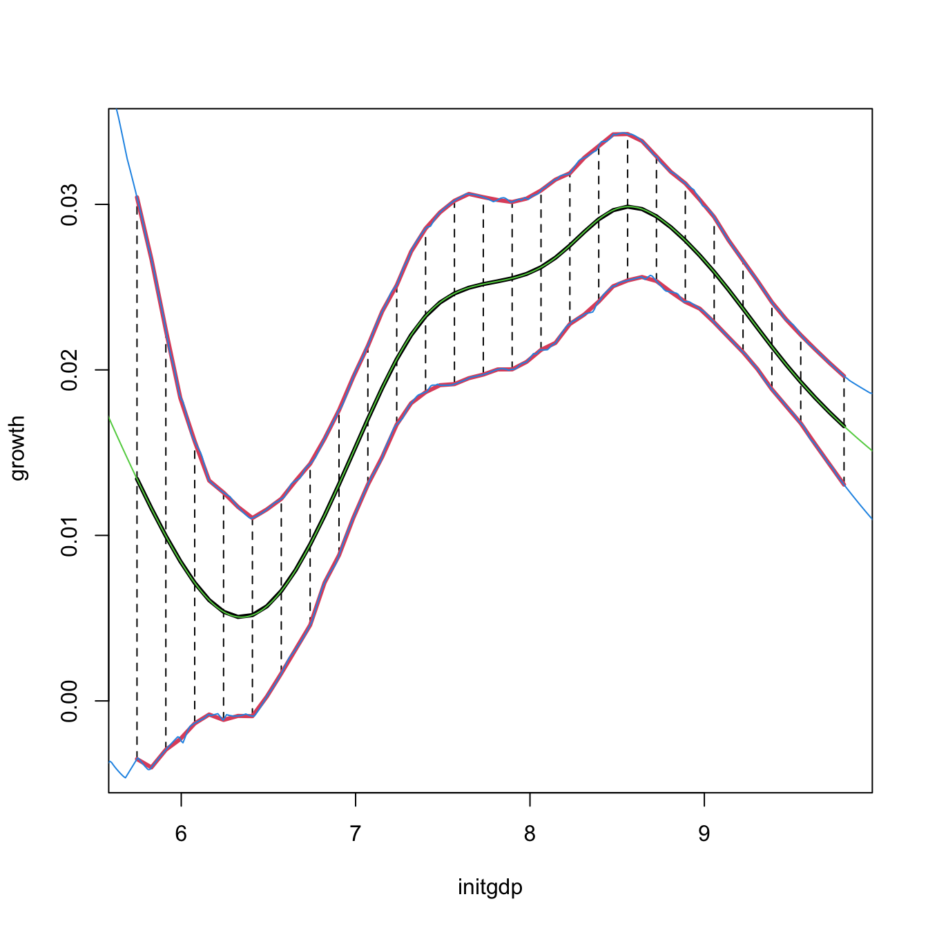
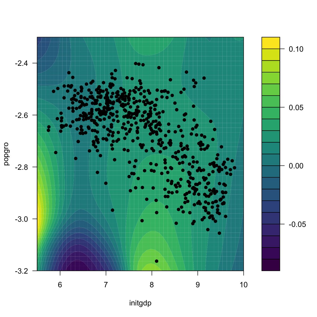
# But np_pred_CI is also valid for regression models with several predictors!
# An example with bivariate local linear regression with CV bandwidth
bw2 <- np::npregbw(formula = growth ~ initgdp + popgro, data = oecdpanel,
                   regtype = "ll")
fit2 <- np::npreg(bw2)

# Predictions and confidence intervals along a bivariate grid
L <- 50
x_initgdp <- seq(5.5, 10, l = L)
x_popgro <- seq(-3.2, -2.3, l = L)
exdat <- expand.grid(x_initgdp, x_popgro)
ci2 <- np_pred_CI(npfit = fit2, exdat = exdat)

# Regression surface. Observe the extrapolatory artifacts for
# low-density regions
m_hat <- matrix(ci2$m_hat, nrow = L, ncol = L)
filled.contour(x_initgdp, x_popgro, m_hat, nlevels = 20,
               color.palette = viridis::viridis,
               xlab = "initgdp", ylab = "popgro",
               plot.axes = {
                 axis(1); axis(2);
                 points(popgro ~ initgdp, data = oecdpanel, pch = 16)
                 })
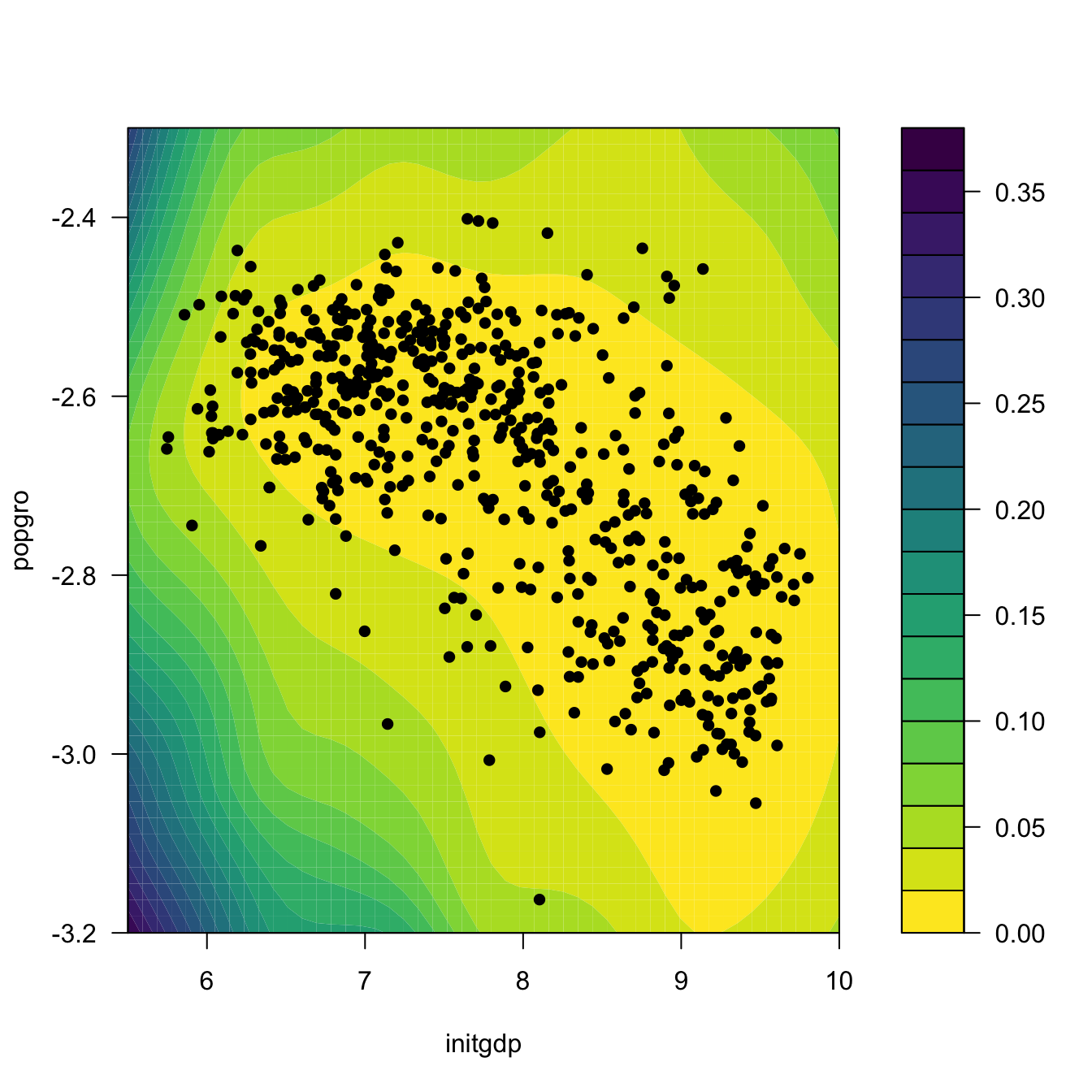
# Length of the 95%-confidence intervals for the regression. Observe how
# they grow for low-density regions
ci_dif <- matrix(ci2$upr - ci2$lwr, nrow = L, ncol = L)
filled.contour(x_initgdp, x_popgro, ci_dif, nlevels = 20,
               color.palette = function(n) viridis::viridis(n, direction = -1),
               xlab = "initgdp", ylab = "popgro",
               plot.axes = {
                 axis(1); axis(2);
                 points(popgro ~ initgdp, data = oecdpanel, pch = 16)
                 })
Exercise 5.8 Split the data(Auto, package = "ISLR") dataset by taking set.seed(12345); ind_train <- sample(nrow(Auto), size = nrow(Auto) - 12) as the index for the training dataset and use the remaining observations for the validation dataset. Then, for the regression problem described in Exercise 5.5:
- Fit the local constant and linear estimators with CV bandwidths by taking the nature of the variables into account. Hint: remember using
orderedandfactorif necessary. - Interpret the nonparametric fits via marginal effects (for the quantile \(0.5\)) and bootstrap confidence intervals.
- Obtain the mean squared prediction error on the validation dataset for the two fits. Which estimate gives the lowest error?
- Compare the errors with the ones made by a linear estimation. Which approach gives lowest errors?
Exercise 5.9 The data(ChickWeight) dataset in R contains \(578\) observations of the weight, Time, and Diet of chicks. Consider the regression weight ~ Time + Diet.
- Fit the local linear estimator with CV bandwidths by taking the nature of the variables into account.
- Plot the marginal effects of
Timefor the four possible types ofDiet. Overlay the four samples and use different colors. Explain your interpretations. - Obtain the bootstrap \(90\%\)-confidence intervals of the expected weight of a chick on the 20th day, for each of the four types of diets (take \(B=500\)). With a \(90\%\) confidence, state which diet dominates in terms of weight the other diets, and which are comparable.
- Produce a plot that shows the extrapolation of the expected weight, for each of the four diets, from the 20th to the 30th day. Add bootstrap \(90\%\)-confidence bands. Explain your interpretations.
Exercise 5.10 Investigate the accuracy of the confidence intervals implemented in np::npplot for a fixed bandwidth \(h\). To do so:
- Simulate \(M=500\) samples of size \(n=100\) from the regression model \(Y=m(X)+\varepsilon,\) where \(m(x) = 0.25x^2 - 0.75x + 3,\) \(X\sim\mathcal{N}(0,1.5^2),\) and \(\varepsilon\sim\mathcal{N}(0,0.75^2).\)
- Compute the \(95\%\)-confidence intervals for \(m(x)\) along
x <- seq(-5, 5, by = 0.1), for each of the \(M\) samples. Do it for the normal approximation and quantile-based confidence intervals. - Check if \(m(x)\) belongs to each of the confidence intervals, for each \(x.\)
- Approximate the actual coverage of the confidence intervals, for each \(x.\)
Once you have a working solution, increase \(n\) to \(n=200,500,\) consider other regression models \(m,\) and summarize your conclusions. Explore the effect of different bandwidth values. Use \(B=500.\)
Naive bootstrap, although conceptually simple, does not capture the uncertainty of \(\hat{m}(\mathbf{x};q,\mathbf{h})\) in all situations, and may severely underestimate the variability of \(\hat{m}(\mathbf{x};q,\mathbf{h}).\) A more sophisticated bootstrap procedure is the so-called wild bootstrap (Wu 1986; Liu 1988; Hardle and Marron 1991), as it is a resampling strategy particularly well-suited for regression problems with heteroscedasticity. The wild bootstrap approach replaces Step 2 in the previous bootstrap resampling with:
- Simulate \(V_1^{*b},\ldots,V_n^{*b}\) to be iid copies of \(V\) such that \(\mathbb{E}[V]=0\) and \(\mathbb{V}\mathrm{ar}[V]=1.\)188
- Compute the perturbed residuals \(\varepsilon_i^{*b}:=\hat\varepsilon_iV_i^{*b},\) where \(\hat\varepsilon_i:=Y_i-\hat{m}(\mathbf{X}_i;q,\mathbf{h}),\) \(i=1,\ldots,n.\)
- Obtain the bootstrap sample \((\mathbf{X}_1,Y_1^{*b}),\ldots,(\mathbf{X}_n,Y_n^{*b}),\) where \(Y_i^{*b}:=\hat{m}(\mathbf{X}_i;q,\mathbf{h})+\varepsilon_i^{*b},\) \(i=1,\ldots,n.\)
- Compute \(\hat{m}^{*b}(\mathbf{x};q,\mathbf{h})=\sum_{i=1}^n W_i^{q}(\mathbf{x})Y_i^{*b}\) from \((\mathbf{X}_1,Y_1^{*b}),\ldots,(\mathbf{X}_n,Y_n^{*b}).\)
Unfortunately, np does not seem to implement the wild bootstrap. The next exercise points to its implementation.
Exercise 5.11 Adapt the np_pred_CI function to include the argument type_boot, which can take either the value "naive" or "wild". If type_boot = "wild", then the function must compute wild bootstrap confidence intervals, implementing from scratch Steps i–iv of the wild bootstrap resampling. Validate the correct behavior of the wild bootstrap confidence intervals in the simulation study described in Exercise 5.10, but considering a single sample size \(n\) and regression model \(m.\)
References
Precisely, the ones associated with the asymptotic normality of \(\hat{m}(\mathbf{x};q,\mathbf{h})\) and that are collected in Theorem 4.2 for the case of a single continuous predictor.↩︎
As usable asymptotic approximations are hampered by two factors: (i) the slow convergence speed towards the asymptotic distribution (recall the effective sample size in Theorem 4.2); and (ii) the need to estimate the unknown terms in the asymptotic bias and variance, which leads to an endless cycle (similar to that in Section 2.4.1).↩︎
This is the same as randomly accessing \(n\) times the rows of the matrix \(\begin{pmatrix} X_{11} & \ldots & X_{1p} & Y_1 \\ \vdots & \ddots & \vdots & \vdots \\ X_{n1} & \ldots & X_{np} & Y_n \end{pmatrix}_{n\times(p+1)}.\)↩︎
Although this might be confusing, since Hayfield and Racine (2008) states that “Specifying the type of bootstrapping as ‘
inid’ admits general heteroscedasticity of unknown form via the wild bootstrap (Liu 1988), though it does not allow for dependence.” but, as of version 0.60-10, the naive bootstrap is run whenplot.errors.boot.method = "inid"(see code).↩︎For example, the golden section binary variable defined by \(\mathbb{P}[V=1-\phi]=p\) and \(\mathbb{P}[V=\phi]=1-p,\) with \(\phi=(1+\sqrt{5})/2\) and \(p=(\phi+2)/5.\)↩︎