2.5 Practical issues

In this section we discuss several practical issues for kernel density estimation.

2.5.1 Boundary issues and transformations

In Section 2.3 we assumed certain regularity conditions for $f.$ Assumption A1 stated that $f$ should be twice continuously differentiable (on $\mathbb{R}$ !). It is simple to think a counterexample to that: take any density with a support with boundary, for example a $\mathcal{LN}(0,1)$ in $(0,\infty),$ as seen below. The kde will run into trouble!

# Sample from a LN(0, 1)
set.seed(123456)
samp <- rlnorm(n = 500)

# kde and density
plot(density(samp), ylim = c(0, 0.8))
curve(dlnorm(x), from = -2, to = 10, n = 500, col = 2, add = TRUE)
rug(samp)

What is happening is clear: the kde is spreading probability mass outside the support of $\mathcal{LN}(0,1),$ because the kernels are functions defined in $\mathbb{R}.$ Since the kde places probability mass at negative values, it takes it from the positive side, resulting in a severe negative bias about the right-hand side of $0.$ As a consequence, the kde does not integrate one in the support of the data. No matter what the sample size considered is, the kde will always have a negative bias of $O(h)$ at the boundary, instead of the standard $O(h^2).$

A simple approach to deal with the boundary bias is to map a non-real-supported density $f$ into a real-supported density $g,$ which is simpler to estimate, by means of a transformation $t$ :

$\begin{align*} f(x)=g(t(x))t'(x). \end{align*}$

The transformation kde is obtained by replacing $g$ with the usual kde, but acting on the transformed data $t(X_1),\ldots,t(X_n)$ :

$\begin{align} \hat{f}_\mathrm{T}(x;h,t):=\frac{1}{n}\sum_{i=1}^nK_h(t(x)-t(X_i))t'(x). \tag{2.34} \end{align}$

Note that $h$ is in the scale of $t(X_i),$ not $X_i.$ Hence, another benefit of this approach, in addition to its simplicity, is that bandwidth selection can be done transparently⁵⁰ in terms of the already discussed bandwidth selectors: select a bandwidth from $t(X_1),\ldots,t(X_n)$ and use it in (2.34). A table with some common transformations⁵¹ is the following.

Transform.	Data in	$t(x)$	$t'(x)$
Log	$(a,\infty)$	$\log(x-a)$	$\frac{1}{x-a}$
Probit	$(a,b)$	$\Phi^{-1}\left(\frac{x-a}{b-a}\right)$	${(b-a)\phi\left(\frac{\Phi^{-1}(x)-a}{b-a}\right)^{-1}}$
Shifted power	$(-\lambda_1,\infty)$ (data skewed)	${(x+\lambda_1)^{\lambda_2}\mathrm{sign}(\lambda_2)}$ if $\lambda_2\neq0$	${\lambda_2(x+\lambda_1)^{\lambda_2-1}\mathrm{sign}(\lambda_2)}$ if $\lambda_2\neq0$

Figure 2.12: Construction of the transformation kde for the log and probit transformations. The left panel shows the kde (2.7) applied to the transformed data. The right plot shows the transformed kde (2.34) applied to the original data. Application available here.

The code below illustrates how to compute a transformation kde in practice from density.

# kde with log-transformed data
kde <- density(log(samp))
plot(kde, main = "Kde of transformed data")
rug(log(samp))


# Careful: kde$x is in the reals!
range(kde$x)
## [1] -4.542984  3.456035

# Untransform kde$x so the grid is in (0, infty)
kde_transf <- kde
kde_transf$x <- exp(kde_transf$x)

# Transform the density using the chain rule
kde_transf$y <- kde_transf$y * 1 / kde_transf$x

# Transformed kde
plot(kde_transf, main = "Transformed kde", xlim = c(0, 15))
curve(dlnorm(x), col = 2, add = TRUE, n = 500)
rug(samp)

Exercise 2.20 Consider the data given by set.seed(12345); x <- rbeta(n = 500, shape1 = 2, shape2 = 2). Compute:

The untransformed kde employing the DPI and LSCV selectors. Overlay the true density.
The transformed kde employing a probit transformation and using the DPI and LSCV selectors on the transformed data.

Exercise 2.21 (Exercise 2.23 in Wand and Jones (1995)) Show that the bias and variance for the transformation kde (2.34) are

$\begin{align*} \mathrm{Bias}[\hat{f}_\mathrm{T}(x;h,t)]&=\frac{1}{2}\mu_2(K)g''(t(x))t'(x)h^2+o(h^2),\\ \mathbb{V}\mathrm{ar}[\hat{f}_\mathrm{T}(x;h,t)]&=\frac{R(K)}{nh}g(t(x))t'(x)^2+o((nh)^{-1}), \end{align*}$

where $g$ is the density of $t(X).$

Exercise 2.22 Using the results from Exercise 2.21, prove that

$\begin{align*} \mathrm{AMISE}[\hat{f}_\mathrm{T}(\cdot;h,t)]=&\,\frac{1}{4}\mu_2^2(K)\int (g''(x))^2t'(t^{-1}(x))\,\mathrm{d}xh^4\\ &+\frac{R(K)}{nh}\mathbb{E}[t'(X)], \end{align*}$

where $g$ is the density of $t(X).$

2.5.2 Sampling

Sampling a kde is relatively straightforward. The trick is to recall

$\begin{align*} \hat{f}(x;h)=\frac{1}{n}\sum_{i=1}^nK_h(x-X_i) \end{align*}$

as a mixture density made of $n$ mixture components in which each of them is sampled independently. The only part that might require special treatment is sampling from the density $K,$ although R contains specific sampling functions for the most popular kernels.

The algorithm for sampling $N$ points goes as follows:

Choose $i\in\{1,\ldots,n\}$ at random.
Sample from $K_h(\cdot-X_i)=\frac{1}{h}K\left(\frac{\cdot-X_i}{h}\right).$
Repeat the previous steps $N$ times.

Let’s see a quick example.

# Sample the claw
n <- 100
set.seed(23456)
samp <- nor1mix::rnorMix(n = n, obj = nor1mix::MW.nm10)

# Kde
h <- 0.1
plot(density(samp, bw = h), main = "", col = 4)

# # Naive sampling algorithm
# N <- 1e6
# samp_kde <- numeric(N)
# for (k in 1:N) {
#
#   i <- sample(x = 1:n, size = 1)
#   samp_kde[k] <- rnorm(n = 1, mean = samp[i], sd = h)
#
# }

# Sample N points from the kde
N <- 1e6
i <- sample(x = n, size = N, replace = TRUE)
samp_kde <- rnorm(N, mean = samp[i], sd = h)

# Add kde of the sampled kde -- almost equal
lines(density(samp_kde), col = 3)
legend("topright", legend = c("Kde", "Kde of sampled kde"),
       lwd = 2, col = 4:3)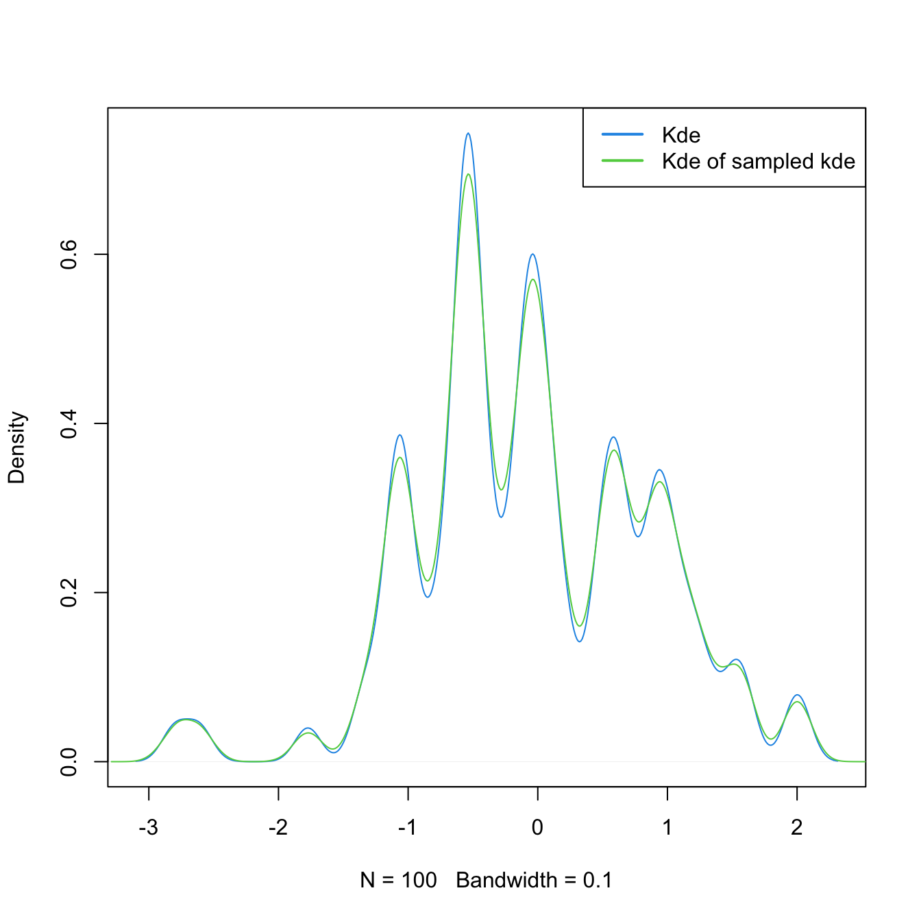

Exercise 2.23 Sample data points from the kde of iris$Petal.Width that is computed with the NS selector.

Exercise 2.24 The dataset sunspot.year contains the yearly numbers of sunspots from 1700 to 1988 (rounded to one digit). Employing a log-transformed kde with DPI bandwidth, sample new sunspots observations. Check by simulation that the sampling is done appropriately by comparing the log-transformed kde of the sampled data with the original kde.

References

Wand, M. P., and M. C. Jones. 1995. Kernel Smoothing. Vol. 60. Monographs on Statistics and Applied Probability. London: Chapman & Hall. https://doi.org/10.1201/b14876.

However, note that the optimality on selecting a bandwidth for estimating $g$ from $t(X_1),\ldots,t(X_n)$ may not translate into an optimality for estimating $f.$ ↩︎
If $\lambda_2\to0$ in the shifted power, then the log transformation follows with $a=-\lambda_1.$ ↩︎