4.3 Bandwidth selection

Bandwidth selection, as for kernel density estimation, is of key practical importance for kernel regression estimation. Several bandwidth selectors have been proposed for kernel regression by following plug-in and cross-validatory ideas that are similar to the ones seen in Section 2.4. For the sake of simplicity, we first briefly overview the plug-in analogues for local linear regression for a single continuous predictor. Then, the main focus will be placed on Least Squares Cross-Validation (LSCV; simply referred to as CV), as the cross-validation methodology readily generalizes to the more complex settings to be seen in Section 5.1.

As in the kde case, the first step for performing bandwidth selection is to define an error criterion suitable for the estimator \(\hat{m}(\cdot;p,h).\) The density-weighted ISE of \(\hat{m}(\cdot;p,h),\)

\[\begin{align*} \mathrm{ISE}[\hat{m}(\cdot;p,h)]:=&\,\int(\hat{m}(x;p,h)-m(x))^2f(x)\,\mathrm{d}x, \end{align*}\]

is often considered. Observe that this definition is very similar to the kde’s ISE, except for the fact that \(f\) appears weighting the quadratic difference: what matters is to minimize the estimation error on the regions where the density of \(X\) is higher. As a consequence, this definition does not give any importance to the errors made by \(\hat{m}(\cdot;p,h)\) when estimating \(m\) at regions with virtually no data.¹⁴⁶

The ISE of \(\hat{m}(\cdot;p,h)\) is a random quantity that directly depends on the sample \((X_1,Y_1),\ldots,(X_n,Y_n).\) In order to avoid this nuisance, the conditional¹⁴⁷ MISE of \(\hat{m}(\cdot;p,h)\) is often employed:

\[\begin{align*} \mathrm{MISE}[\hat{m}(\cdot;p,h)&|X_1,\ldots,X_n]\\ :=&\,\mathbb{E}\left[\mathrm{ISE}[\hat{m}(\cdot;p,h)]|X_1,\ldots,X_n\right]\\ =&\,\int\mathbb{E}\left[(\hat{m}(x;p,h)-m(x))^2|X_1,\ldots,X_n\right]f(x)\,\mathrm{d}x\\ =&\,\int\mathrm{MSE}\left[\hat{m}(x;p,h)|X_1,\ldots,X_n\right]f(x)\,\mathrm{d}x. \end{align*}\]

Clearly, the goal is to find the bandwidth that minimizes this error,

\[\begin{align*} h_\mathrm{MISE}:=\arg\min_{h>0}\mathrm{MISE}[\hat{m}(\cdot;p,h)|X_1,\ldots,X_n], \end{align*}\]

but this is an untractable problem because of the lack of explicit expressions. However, since the MISE follows by integrating the conditional MSE, explicit asymptotic expressions can be found.

In the case of local linear regression, the conditional MSE follows by the conditional squared bias (4.16) and the variance (4.17) given in Theorem 4.1. This produces the conditional AMISE for \(\hat{m}(\cdot;p,h),\) \(p=0,1\):

\[\begin{align} \mathrm{AMISE}[\hat{m}(\cdot;p,h)|X_1,\ldots,X_n]=&\,h^4\int B_p(x)^2f(x)\,\mathrm{d}x\nonumber\\ &+\frac{R(K)}{nh}\int\sigma^2(x)\,\mathrm{d}x.\tag{4.20} \end{align}\]

If \(p=1,\) the resulting optimal AMISE bandwidth is

\[\begin{align} h_\mathrm{AMISE}=\left[\frac{R(K)\int\sigma^2(x)\,\mathrm{d}x}{\mu_2^2(K)\theta_{22}(m)n}\right]^{1/5},\tag{4.21} \end{align}\]

where

\[\begin{align*} \theta_{22}(m):=\int(m''(x))^2f(x)\,\mathrm{d}x \end{align*}\]

acts as the “density-weighted curvature of \(m\)” and completely resembles the curvature term \(R(f'')\) that appeared in Section 2.4.

Exercise 4.11 Obtain \(\mathrm{AMISE}[\hat{m}(\cdot;p,h)|X_1,\ldots,X_n]\) in (4.20) from Theorem 4.1.

Exercise 4.12 Obtain the expression for \(h_\mathrm{AMISE}\) in (4.21) from \(\mathrm{AMISE}[\hat{m}(\cdot;1,h)|X_1,\ldots,X_n].\) Then, obtain the corresponding AMISE optimal bandwidth for \(\hat{m}(\cdot;0,h).\)

As happened in the density setting, the AMISE-optimal bandwidth can not be readily employed, as knowledge about the curvature of \(m,\) \(\theta_{22}(m),\) is required. To make things worse, (4.21) also depends on the integrated conditional variance \(\int\sigma^2(x)\,\mathrm{d}x,\) which is unknown too.

4.3.1 Plug-in rules

A possibility to estimate \(\theta_{22}(m)\) and \(\int\sigma^2(x)\,\mathrm{d}x,\) in the spirit of the normal scale bandwidth selector (or zero-stage plug-in selector) seen in Section 2.4.1, is presented in Section 4.2 in Fan and Gijbels (1996). There, a global parametric fit based on a fourth-order¹⁴⁸ polynomial is employed:

\[\begin{align*} \hat{m}_Q(x)=\hat{\alpha}_0+\sum_{j=1}^4\hat{\alpha}_jx^j, \end{align*}\]

where \(\hat{\boldsymbol{\alpha}}\) is obtained from \((X_1,Y_1),\ldots,(X_n,Y_n).\) The second derivative of this quartic fit is

\[\begin{align*} \hat{m}_Q''(x)=2\hat{\alpha}_2+6\hat{\alpha}_3x+12\hat{\alpha}_4x^2. \end{align*}\]

Besides, \(\theta_{22}(m)\) can be written in terms of an expectation, which motivates its estimation by Monte Carlo:

\[\begin{align*} \theta_{22}(m)=\mathbb{E}[(m''(X))^2]\approx\frac{1}{n}\sum_{i=1}^n(m''(X_i))^2=:\hat{\theta}_{22}(m). \end{align*}\]

Therefore, combining both estimations we can substitute \(\theta_{22}(m)\) with \(\hat{\theta}_{22}(\hat{m}_Q)\) in (4.21).

It remains to estimate \(\int\sigma^2(x)\,\mathrm{d}x,\) which we can do by assuming homoscedasticity and then estimating the common variance by¹⁴⁹

\[\begin{align*} \hat{\sigma}_Q^2:=\frac{1}{n-5}\sum_{i=1}^n(Y_i-\hat{m}_Q(X_i))^2. \end{align*}\]

In addition, if we assume that the variance is zero outside the support of \(X\) (where there is no data), we can replace \(\int\sigma^2(x)\,\mathrm{d}x\) with the estimate \((X_{(n)}-X_{(1)})\hat{\sigma}_Q^2\,\)¹⁵⁰ and obtain the Rule-of-Thumb bandwidth selector (RT)

\[\begin{align*} \hat{h}_\mathrm{RT}=\left[\frac{R(K)(X_{(n)}-X_{(1)})\hat{\sigma}_Q^2}{\mu_2^2(K)\hat{\theta}_{22}(\hat{m}_Q)n}\right]^{1/5}. \end{align*}\]

The following code illustrates how to implement this simple selector.

# Evaluation grid
x_grid <- seq(0, 5, l = 500)

# Quartic-like regression function
m <- function(x) 5 * dnorm(x, mean = 1.5, sd = 0.25) - x

# # Highly nonlinear regression function
# m <- function(x) x * sin(2 * pi * x)

# # Quartic regression function (but expressed in a orthogonal polynomial)
# coefs <- attr(poly(x_grid / 5 * 3, degree = 4), "coefs")
# m <- function(x) 20 * poly(x, degree = 4, coefs = coefs)[, 4]

# # Seventh orthogonal polynomial
# coefs <- attr(poly(x_grid / 5 * 3, degree = 7), "coefs")
# m <- function(x) 20 * poly(x, degree = 7, coefs = coefs)[, 7]

# Generate some data
set.seed(123456)
n <- 250
eps <- rnorm(n)
X <- abs(rnorm(n))
Y <- m(X) + eps

# Rule-of-thumb selector
h_RT <- function(X, Y) {

  # Quartic fit
  mod_Q <- lm(Y ~ poly(X, raw = TRUE, degree = 4))

  # Estimates of unknown quantities
  int_sigma2_hat <- diff(range(X)) * sum(mod_Q$residuals^2) / mod_Q$df.residual
  theta_22_hat <- mean((2 * mod_Q$coefficients[3] +
                        6 * mod_Q$coefficients[4] * X +
                        12 * mod_Q$coefficients[5] * X^2)^2)

  # h_RT
  R_K <- 0.5 / sqrt(pi)
  ((R_K * int_sigma2_hat) / (theta_22_hat * length(X)))^(1 / 5)

}

# Selected bandwidth
(h_ROT <- h_RT(X = X, Y = Y))
## [1] 0.1111711

# Local linear fit
lp1_RT <- KernSmooth::locpoly(x = X, y = Y, bandwidth = h_ROT, degree = 1,
                              range.x = c(0, 10), gridsize = 500)

# Quartic fit employed
mod_Q <- lm(Y ~ poly(X, raw = TRUE, degree = 4))

# Plot data
plot(X, Y, ylim = c(-6, 8))
rug(X, side = 1); rug(Y, side = 2)
lines(x_grid, m(x_grid), col = 1)
lines(lp1_RT$x, lp1_RT$y, col = 2)
lines(x_grid, mod_Q$coefficients[1] +
        poly(x_grid, raw = TRUE, degree = 4) %*% mod_Q$coefficients[-1],
      col = 3)
legend("topright", legend = c("True regression", "Local linear (RT)",
                              "Quartic fit"),
       lwd = 2, col = 1:3)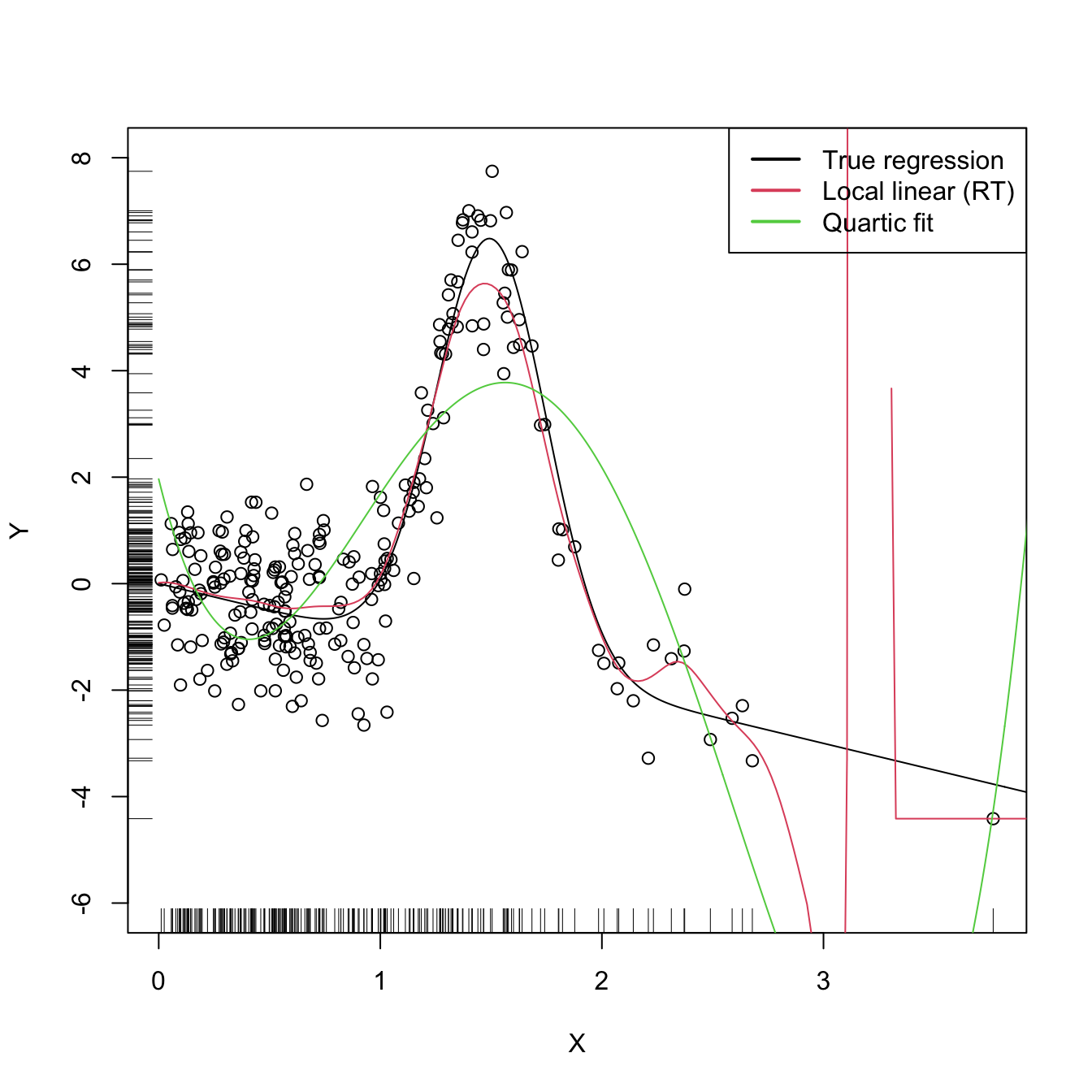

Figure 4.3: Local linear estimator with \(\hat{h}_\mathrm{RT}\) bandwidth and the quartic global fit. Observe how the local linear estimator behaves erratically at regions with no data – a fact due to the strong dependence of the locally weighted linear regression on few observations.

The \(\hat{h}_\mathrm{RT}\) selector strongly depends on how well the curvature of \(m\) is approximated by the quartic fit. In addition, it assumes that the conditional variance is constant, which may be unrealistic. The exercise below intends to illustrate these limitations.

Exercise 4.13 Explore in the code above the effect of the regression function, and visualize how poor quartic fits tend to give poor nonparametric fits. Then, adapt the sampling mechanism to introduce heteroskedasticity on \(Y\) and investigate the behavior of the nonparametric estimator based on \(\hat{h}_\mathrm{RT}.\)

The rule-of-thumb selector is a zero-stage plug-in selector. An \(\ell\)-stage plug-in selector was proposed by Ruppert, Sheather, and Wand (1995)¹⁵¹ and shares the same spirit of the DPI bandwidth selector seen in Section 2.4.1. As a consequence, the DPI selector for kre turns (4.21) into an usable selector by following a known agenda: it employs a series of optimal nonparametric estimations of \(\theta_{22}(m)\) that depend on high-order curvature terms \(\theta_{rs}(m):=\int m^{(r)}(x)m^{(s)}(x)f(x)\,\mathrm{d}x,\) ending this iterative procedure with a parametric estimation of a higher-order curvature.

The kind of parametric fit employed is a “block quartic fit”. This is a series of \(N\) different quartic fits \(\hat{m}_{Q,1},\ldots,\hat{m}_{Q,N}\) of the regression function \(m\) that are done in \(N\) blocks of the data. These blocks are defined by sorting the sample \(X_1,\ldots,X_n\) and then partitioning it into approximately \(N\) blocks of equal size \(n/N.\) The purpose of the block quartic fit is to achieve more flexibility on the estimation of the curvature¹⁵² terms \(\theta_{22}(m)\) and \(\theta_{24}(m).\) The estimation of \(\int\sigma^2(x)\,\mathrm{d}x\) is carried out by pooling the individual estimates of the conditional variance in the \(N\) blocks, \(\hat{\sigma}^2_{Q,1},\ldots,\hat{\sigma}^2_{Q,N},\) and by assuming a compactly supported density \(f.\)¹⁵³ The selection of \(N\) can be done in a data-driven way by relying on a model selection criterion (see Ruppert, Sheather, and Wand (1995)), such as the AIC or BIC.

The resulting bandwidth selector, \(\hat{h}_\mathrm{DPI},\) has a much faster convergence rate to \(h_{\mathrm{MISE}}\) than cross-validatory selectors. However, it is notably more convoluted, and as a consequence it is less straightforward to extend to more complex settings.¹⁵⁴

The DPI selector for the local linear estimator is implemented in KernSmooth::dpill.

# Generate some data
set.seed(123456)
n <- 250
eps <- rnorm(n)
X <- abs(rnorm(n))
m <- function(x) x * sin(2 * pi * x)
Y <- m(X) + eps

# Selected bandwidth
(h_ROT <- h_RT(X = X, Y = Y))
## [1] 0.3489934

# DPI selector
(h_DPI <- KernSmooth::dpill(x = X, y = Y))
## [1] 0.05172781

# Fits
lp1_RT <- KernSmooth::locpoly(x = X, y = Y, bandwidth = h_ROT, degree = 1,
                              range.x = c(0, 10), gridsize = 500)
lp1_DPI <- KernSmooth::locpoly(x = X, y = Y, bandwidth = h_DPI, degree = 1,
                               range.x = c(0, 10), gridsize = 500)

# Plot data
plot(X, Y, ylim = c(-6, 8))
rug(X, side = 1); rug(Y, side = 2)
lines(x_grid, m(x_grid), col = 1)
lines(lp1_DPI$x, lp1_DPI$y, col = 2)
lines(lp1_RT$x, lp1_RT$y, col = 3)
legend("topleft", legend = c("True regression", "Local linear (DPI)",
                             "Local linear (RT)"), lwd = 2, col = 1:3)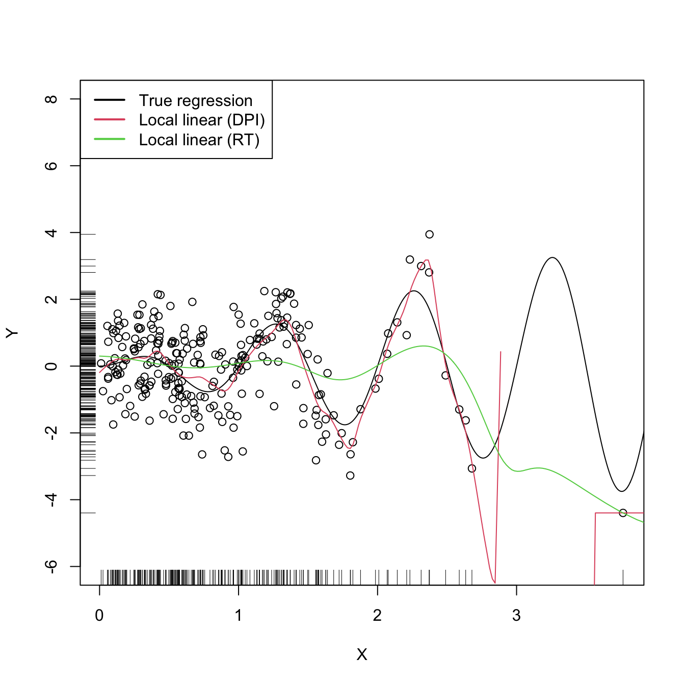

4.3.2 Cross-validation

Following an analogy with the fit of the linear model (see Section B.1.1), an obvious possibility is to select an adequate bandwidth \(h\) for \(\hat{m}(\cdot;p,h)\) that minimizes a Residual Sum of Squares (RSS) of the form

\[\begin{align} \frac{1}{n}\sum_{i=1}^n(Y_i-\hat{m}(X_i;p,h))^2.\tag{4.22} \end{align}\]

However, this is a bad idea. Contrarily to what happened in the linear model, where it was almost¹⁵⁵ impossible to perfectly fit the data due to the limited flexibility of the model, the infinite flexibility of the local polynomial estimator allows interpolating the data if \(h\to0.\) As a consequence, attempting to minimize (4.22) always leads to \(h\approx 0,\) which results in a useless interpolation that misses the target of the estimation, \(m.\)

# Grid for representing (4.22)
h_grid <- seq(0.1, 1, l = 200)^2
error <- sapply(h_grid, function(h) {
  mean((Y - nw(x = X, X = X, Y = Y, h = h))^2)
})

# Error curve
plot(h_grid, error, type = "l")
rug(h_grid)
abline(v = h_grid[which.min(error)], col = 2)

The root of the problem is the comparison of \(Y_i\) with \(\hat{m}(X_i;p,h),\) since there is nothing that forbids that, when \(h\to0,\) \(\hat{m}(X_i;p,h)\to Y_i.\) We can change this behavior if we compare \(Y_i\) with \(\hat{m}_{-i}(X_i;p,h)\,\)¹⁵⁶, the leave-one-out estimate of \(m\) computed without the \(i\)-th datum \((X_i,Y_i),\) yielding the least squares cross-validation error

\[\begin{align} \mathrm{CV}(h):=\frac{1}{n}\sum_{i=1}^n(Y_i-\hat{m}_{-i}(X_i;p,h))^2\tag{4.23} \end{align}\]

and then choose

\[\begin{align*} \hat{h}_\mathrm{CV}:=\arg\min_{h>0}\mathrm{CV}(h). \end{align*}\]

The optimization of (4.23) might seem to be very expensive computationally, since computing \(n\) regressions for just a single evaluation of the cross-validation function is required. There is, however, a simple and neat theoretical result that vastly reduces the computational complexity, at the price of increasing the memory demand. This trick allows computing, with a single fit, the cross-validation function evaluated at \(h.\)

Proposition 4.1 For any \(p\geq0,\) the weights of the leave-one-out estimator \(\hat{m}_{-i}(x;p,h)=\sum_{\substack{j=1\\j\neq i}}^nW_{-i,j}^p(x)Y_j\) can be obtained from \(\hat{m}(x;p,h)=\sum_{i=1}^nW_{i}^p(x)Y_i\):

\[\begin{align} W_{-i,j}^p(x)=\frac{W^p_j(x)}{\sum_{\substack{k=1\\k\neq i}}^nW_k^p(x)}=\frac{W^p_j(x)}{1-W_i^p(x)}.\tag{4.24} \end{align}\]

This implies that

\[\begin{align} \mathrm{CV}(h)=\frac{1}{n}\sum_{i=1}^n\left(\frac{Y_i-\hat{m}(X_i;p,h)}{1-W_i^p(X_i)}\right)^2.\tag{4.25} \end{align}\]

The result can be proved by recalling that \(\hat{m}(x;p,h)\) is a linear combination¹⁵⁷ of the responses \(\{Y_i\}_{i=1}^n.\)

Exercise 4.14 Consider the Nadaraya–Watson estimator (\(p=0\)). Then, show (4.24) using (4.14). From there, conclude the proof of Proposition 4.1.

Exercise 4.15 Prove the second equality in (4.24) for the local linear estimator (\(p=1\)). From there, prove (4.25). Use (4.15).

Remark. Observe that computing (4.25) requires evaluating the local polynomial estimator at the sample \(\{X_i\}_{i=1}^n\) and obtaining \(\{W_i^p(X_i)\}_{i=1}^n\) (which are needed to evaluate \(\hat{m}(X_i;p,h)\)). Both tasks can be achieved simultaneously from the \(n\times n\) matrix \(\big(W_{i}^p(X_j)\big)_{ij}\) and, if \(p=0,\) directly from the symmetric \(n\times n\) matrix \(\left(K_h(X_i-X_j)\right)_{ij},\) for which the storage cost is \(O((n^2-n)/2)\) (the diagonal is constant).

Let’s implement \(\hat{h}_\mathrm{CV}\) employing (4.25) for the Nadaraya–Watson estimator.

# Generate some data to test the implementation
set.seed(12345)
n <- 200
eps <- rnorm(n, sd = 2)
m <- function(x) x^2 + sin(x)
X <- rnorm(n, sd = 1.5)
Y <- m(X) + eps
x_grid <- seq(-10, 10, l = 500)

# Objective function
cv_nw <- function(X, Y, h, K = dnorm) {

  sum(((Y - nw(x = X, X = X, Y = Y, h = h, K = K)) /
         (1 - K(0) / colSums(K(outer(X, X, "-") / h))))^2)

}

# Find optimum CV bandwidth, with sensible grid
bw_cv_grid <- function(X, Y,
                       h_grid = diff(range(X)) * (seq(0.05, 0.5, l = 200))^2,
                       K = dnorm, plot_cv = FALSE) {

  # Minimize the CV function on a grid
  obj <- sapply(h_grid, function(h) cv_nw(X = X, Y = Y, h = h, K = K))
  h <- h_grid[which.min(obj)]

  # Add plot of the CV loss
  if (plot_cv) {

    plot(h_grid, obj, type = "o")
    rug(h_grid)
    abline(v = h, col = 2, lwd = 2)

  }

  # CV bandwidth
  return(h)

}

# Bandwidth
h <- bw_cv_grid(X = X, Y = Y, plot_cv = TRUE)

h
## [1] 0.3173499

# Plot result
plot(X, Y)
rug(X, side = 1); rug(Y, side = 2)
lines(x_grid, m(x_grid), col = 1)
lines(x_grid, nw(x = x_grid, X = X, Y = Y, h = h), col = 2)
legend("top", legend = c("True regression", "Nadaraya-Watson"),
       lwd = 2, col = 1:2)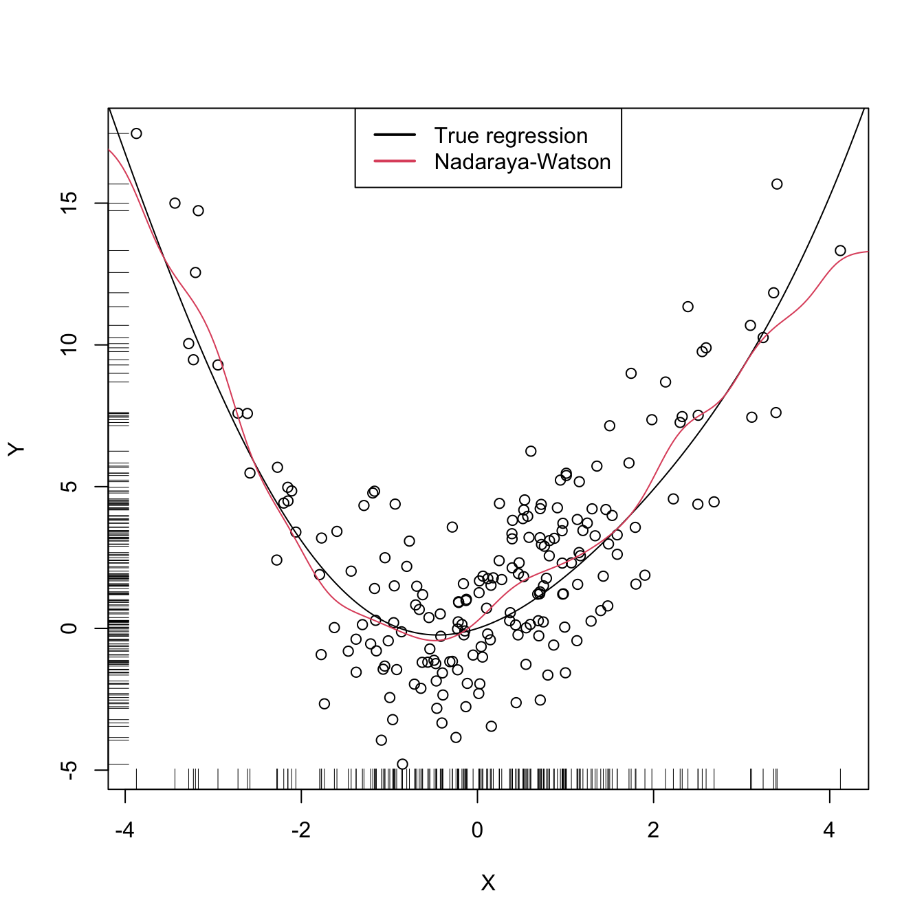

An important warning when computing cross-validation bandwidths is that the objective function can be challenging to minimize and may present several local minima. Therefore, if possible, it is always advisable to graphically inspect the CV loss curve and to run an exhaustive search. When employing an automatic optimization procedure, it is recommended to use several starting values.

The following chunk of code presents the inefficient implementation of \(\hat{h}_\mathrm{CV}\) (based on the definition) and evidences its poorer performance.

# Slow objective function
cv_nw_slow <- function(X, Y, h, K = dnorm) {

  sum((Y - sapply(1:length(X), function(i) {
    nw(x = X[i], X = X[-i], Y = Y[-i], h = h, K = K)
    }))^2)

}

# Optimum CV bandwidth, with sensible grid
bw_cv_grid_slow <- function(X, Y, h_grid =
                              diff(range(X)) * (seq(0.05, 0.5, l = 200))^2,
                            K = dnorm, plot_cv = FALSE) {

  # Minimize the CV function on a grid
  obj <- sapply(h_grid, function(h) cv_nw_slow(X = X, Y = Y, h = h, K = K))
  h <- h_grid[which.min(obj)]

  # Add plot of the CV loss
  if (plot_cv) {

    plot(h_grid, obj, type = "o")
    rug(h_grid)
    abline(v = h, col = 2, lwd = 2)

  }

  # CV bandwidth
  return(h)

}

# Same bandwidth
h <- bw_cv_grid_slow(X = X, Y = Y, plot_cv = TRUE)

h
## [1] 0.3173499

# # Time comparison, a factor 10 difference
# microbenchmark::microbenchmark(bw_cv_grid(X = X, Y = Y),
#                                bw_cv_grid_slow(X = X, Y = Y),
#                                times = 10)

Finally, the following chunk of code illustrates the estimation of the regression function of the weight on the mpg in data(Auto, package = "ISLR"), using a cross-validation bandwidth.

# Data -- nonlinear trend
data(Auto, package = "ISLR")
X <- Auto$weight
Y <- Auto$mpg
plot(X, Y, xlab = "weight", ylab = "mpg", pch = 16)

# CV bandwidth
h <- bw_cv_grid(X = X, Y = Y, plot_cv = TRUE)

h
## [1] 110.0398

# Add regression
x_grid <- seq(1600, 5200, by = 10)
plot(X, Y, xlab = "weight", ylab = "mpg", pch = 16)
rug(X, side = 1); rug(Y, side = 2)
lines(x_grid, nw(x = x_grid, X = X, Y = Y, h = h), col = 2)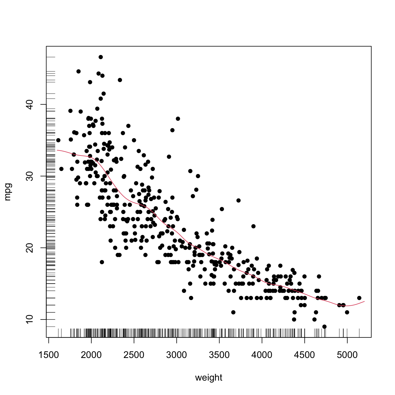

References

Fan, J., and I. Gijbels. 1996. Local Polynomial Modelling and Its Applications. Vol. 66. Monographs on Statistics and Applied Probability. London: Chapman & Hall. https://doi.org/10.1201/9780203748725.

Ruppert, D., S. J. Sheather, and M. P. Wand. 1995. “An Effective Bandwidth Selector for Local Least Squares Regression.” Journal of the American Statistical Association 90 (432): 1257–70. https://doi.org/10.1080/01621459.1995.10476630.

Wand, M. P., and M. C. Jones. 1995. Kernel Smoothing. Vol. 60. Monographs on Statistics and Applied Probability. London: Chapman & Hall. https://doi.org/10.1201/b14876.

---

146. Estimating \(m\) at regions with no data is an extrapolation problem. This kind of estimation makes better sense if a specific structure for \(m\) is assumed (which is not done with a nonparametric estimate of \(m\)), so that this structure can determine the estimate of \(m\) at the regions with no data.↩︎

147. The conditioning is on the sample of the predictor, as it is usually done in a regression setting. The reason why this conditioning is done is to avoid the analysis of the randomness of \(X.\)↩︎

148. In general, a polynomial fit of order \(p+3\) can be considered, but we are restricting to \(p=1.\) The motivation for this order is that it has to be able to estimate the \((p+1)\)-th derivative of \(m\) at \(x,\) \(m^{(p+1)}(x),\) with certain flexibility, and a polynomial fit of order \(p+3\) would be able to do so by a quadratic polynomial.↩︎

149. Notice that the \(n-5\) in the denominator appears because the degrees of freedom of the residuals in a polynomial fit of order \(p+3\) is \(n-p-4,\) and we are considering \(p=1.\) Hence, \(\hat{\sigma}_Q^2\) is an unbiased estimator of \(\sigma_Q^2=\mathbb{V}\mathrm{ar}_Q[Y|X=x]=\mathbb{E}[(Y-m_Q(X))^2|X=x].\)↩︎

150. This is a slightly different adaptation from Fan and Gijbels (1996), where \(\int\sigma^2(x)w_0(x)\,\mathrm{d}x\) is considered and therefore the estimate \(\hat{\sigma}_Q^2\int w_0(x)\,\mathrm{d}x\) naturally follows. This weight \(w_0,\) however, can be an indicator of the support of \(X,\) which gives in that case the selector described here.↩︎

151. See Section 5.8 in Wand and Jones (1995) for a quick introduction.↩︎

152. Notice that this approach does not guarantee the continuity of the final estimate, but since the goal is on estimating the curvature this is not relevant.↩︎

153. So that, if \(\sigma^2(x)\) is constant, \(\int\sigma^2(x)\,\mathrm{d}x\) is finite because we integrate on a compact set.↩︎

154. In particular, the construction of block polynomial fits may be challenging to extend to \(\mathbb{R}^p.\)↩︎

155. Excluding colinear dispositions of the data and assuming that \(n>p.\)↩︎

156. In this case, when \(h\to0,\) \(\hat{m}_{-i}(X_i;p,h)\not\to Y_i\) because \((X_i,Y_i)\) does not belong to the sample employed for computing \(\hat{m}_{-i}(\cdot;p,h).\) Notice that \(\hat{m}_{-i}(X_j;p,h)\to Y_j\) when \(h\to0\) if \(j\neq i,\) but this is not problematic because in \(\sum_{i=1}^n(Y_i-\hat{m}_{-i}(X_i;p,h))^2\) the leave-one-out estimate is different for each \(i=1,\ldots,n.\)↩︎

157. Indeed, for any other linear smoother of the response, the result will also hold.↩︎