5.1 Kernel regression with mixed multivariate data

5.1.1 Multivariate kernel regression

We start by addressing the first generalization:

How to extend the local polynomial estimator $\hat{m}(\cdot;q,h)\,$¹⁶³ to deal with $p$ continuous predictors?

Although this can be done for $q\geq0,$ we focus on the local constant and linear estimators ($q=0,1$) to avoid excessive technical complications.¹⁶⁴

The initial step is to state what the population object to be estimated is, which is now the function $m:\mathbb{R}^p\longrightarrow\mathbb{R}$ given by¹⁶⁵

\[\begin{align} m(x):=\mathbb{E}[Y\vert \mathbf{X}=\mathbf{x}]=\int yf_{Y\vert \mathbf{X}=\mathbf{x}}(y)\,\mathrm{d}y,\tag{5.1} \end{align}\]

where $\mathbf{X}=(X_1,\ldots,X_p)'$ denotes the random vector of the predictors. Hence, despite having a form slightly different from (4.1), (4.1) and (5.1) are conceptually equal. As a consequence, the density-based view¹⁶⁶ of $m$ holds:

\[\begin{align} m(x)=\frac{\int y f(\mathbf{x},y)\,\mathrm{d}y}{f_\mathbf{X}(\mathbf{x})},\tag{5.2} \end{align}\]

where $f$ is the joint density of $(\mathbf{X},Y)$ and $f_\mathbf{X}$ is the marginal pdf of $\mathbf{X}.$

Therefore, given a sample $(\mathbf{X}_1,Y_1),\ldots,(\mathbf{X}_n,Y_n),$ we can estimate $f$ and $f_\mathbf{X},$ analogously to how we did in Section 4.1.1, by the kde’s¹⁶⁷

\[\begin{align} \hat{f}(\mathbf{x},y;\mathbf{H},h)&=\frac{1}{n}\sum_{i=1}^nK_{\mathbf{H}}(\mathbf{x}-\mathbf{X}_{i})K_{h}(y-Y_{i}),\tag{5.3}\\ \hat{f}_\mathbf{X}(\mathbf{x};\mathbf{H})&=\frac{1}{n}\sum_{i=1}^nK_{\mathbf{H}}(\mathbf{x}-\mathbf{X}_{i}).\tag{5.4} \end{align}\]

Plugging these estimators in (5.2), we readily obtain the Nadaraya–Watson estimator for multivariate predictors:

\[\begin{align} \hat{m}(\mathbf{x};0,\mathbf{H}):=\sum_{i=1}^n\frac{K_\mathbf{H}(\mathbf{x}-\mathbf{X}_i)}{\sum_{j=1}^nK_\mathbf{H}(\mathbf{x}-\mathbf{X}_j)}Y_i=\sum_{i=1}^nW^0_{i}(\mathbf{x})Y_i, \tag{5.5} \end{align}\]

where

\[\begin{align*} W^0_{i}(\mathbf{x}):=\frac{K_\mathbf{H}(\mathbf{x}-\mathbf{X}_i)}{\sum_{i=1}^nK_\mathbf{H}(\mathbf{x}-\mathbf{X}_i)}. \end{align*}\]

Exercise 5.1 Derive (5.5) by plugging (5.3) and (5.4) into (5.2).

Usually, to avoid a quick escalation of the number of smoothing bandwidths¹⁶⁸, it is customary to consider product kernels for smoothing $\mathbf{X},$ that is, to consider a diagonal bandwidth $\mathbf{H}=\mathrm{diag}(h_1^2,\ldots,h_p^2)=\mathrm{diag}(\mathbf{h}^2),$ which gives the estimator implemented by the np package:

\[\begin{align*} \hat{m}(\mathbf{x};0,\mathbf{h}):=\sum_{i=1}^nW^0_{i}(\mathbf{x})Y_i \end{align*}\]

where

\[\begin{align*} W^0_{i}(\mathbf{x})&=\frac{K_\mathbf{h}(\mathbf{x}-\mathbf{X}_i)}{\sum_{j=1}^nK_\mathbf{h}(\mathbf{x}-\mathbf{X}_j)},\\ K_\mathbf{h}(\mathbf{x}-\mathbf{X}_i)&=K_{h_1}(x_1-X_{i1})\times\stackrel{p}{\cdots}\times K_{h_p}(x_p-X_{ip}). \end{align*}\]

As in the univariate case, the Nadaraya–Watson estimate can be seen as a weighted average of $Y_1,\ldots,Y_n$ by means of the weights $\{W_i^0(\mathbf{x})\}_{i=1}^n.$ Therefore, the Nadaraya–Watson estimator is a local mean of $Y_1,\ldots,Y_n$ about $\mathbf{X}=\mathbf{x}.$

The derivation of the local linear estimator involves slightly more complex arguments, but analogous to the extension of the linear model from univariate to multivariate predictors. Considering the first-order Taylor expansion

\[\begin{align*} m(\mathbf{X}_i)\approx m(\mathbf{x})+\mathrm{D}m(\mathbf{x})'(\mathbf{X}_i-\mathbf{x}), \end{align*}\]

instead of (4.7) it is possible to arrive to the analogue¹⁶⁹ of (4.10),

\[\begin{align*} \hat{\boldsymbol{\beta}}_\mathbf{h}:=\arg\min_{\boldsymbol{\beta}\in\mathbb{R}^{p+1}}\sum_{i=1}^n\left(Y_i-\boldsymbol{\beta}'(1,(\mathbf{X}_i-\mathbf{x})')'\right)^2K_\mathbf{h}(\mathbf{x}-\mathbf{X}_i), \end{align*}\]

and then solve the problem in the exact same way but now considering the design matrix¹⁷⁰

\[\begin{align*} \mathbf{X}:=\begin{pmatrix} 1 & (\mathbf{X}_1-\mathbf{x})'\\ \vdots & \vdots\\ 1 & (\mathbf{X}_n-\mathbf{x})'\\ \end{pmatrix}_{n\times(p+1)} \end{align*}\]

and

\[\begin{align*} \mathbf{W}:=\mathrm{diag}(K_{\mathbf{h}}(\mathbf{X}_1-\mathbf{x}),\ldots, K_\mathbf{h}(\mathbf{X}_n-\mathbf{x})). \end{align*}\]

The estimate¹⁷¹ for $m(\mathbf{x})$ is therefore obtained from the solution of the weighted least squares problem

\[\begin{align*} \hat{\boldsymbol{\beta}}_{\mathbf{h}}&=\arg\min_{\boldsymbol{\beta}\in\mathbb{R}^{p+1}} (\mathbf{Y}-\mathbf{X}\boldsymbol{\beta})'\mathbf{W}(\mathbf{Y}-\mathbf{X}\boldsymbol{\beta})\\ &=(\mathbf{X}'\mathbf{W}\mathbf{X})^{-1}\mathbf{X}'\mathbf{W}\mathbf{Y} \end{align*}\]

\[\begin{align} \hat{m}(\mathbf{x};1,h):=&\,\hat{\beta}_{\mathbf{h},0}\nonumber\\ =&\,\mathbf{e}_1'(\mathbf{X}'\mathbf{W}\mathbf{X})^{-1}\mathbf{X}'\mathbf{W}\mathbf{Y}\tag{5.6}\\ =&\,\sum_{i=1}^nW^1_{i}(\mathbf{x})Y_i,\nonumber \end{align}\]

where

\[\begin{align*} W^1_{i}(\mathbf{x}):=\mathbf{e}_1'(\mathbf{X}'\mathbf{W}\mathbf{X})^{-1}\mathbf{X}'\mathbf{W}\mathbf{e}_i. \end{align*}\]

Therefore, the local linear estimator is a weighted linear combination of the responses. Differently to the Nadaraya–Watson estimator, this linear combination is not a weighted mean in general, since the weights $W^1_{i}(\mathbf{x})$ can be negative despite $\sum_{i=1}^nW_i^1(\mathbf{x})=1.$

Exercise 5.2 Implement an R function to compute $\hat{m}(\mathbf{x};1,h)$ for an arbitrary dimension $p.$ The function must receive as arguments the sample $(\mathbf{X}_1,Y_1),\ldots,(\mathbf{X}_n,Y_n),$ the bandwidth vector $\mathbf{h},$ and a collection of evaluation points $\mathbf{x}.$ Implement the function by computing the design matrix $\mathbf{X},$ the weight matrix $\mathbf{W},$ the vector of responses $\mathbf{Y},$ and then applying (5.6). Test the implementation in the example below.

The following code performs the local regression estimators with two predictors and exemplifies how the use of np::npregbw and np::npreg is analogous in this bivariate case.

# Sample data from a bivariate regression
n <- 300
set.seed(123456)
X <- mvtnorm::rmvnorm(n = n, mean = c(0, 0),
                      sigma = matrix(c(2, 0.5, 0.5, 1.5), nrow = 2, ncol = 2))
m <- function(x) 0.5 * (x[, 1]^2 + x[, 2]^2)
epsilon <- rnorm(n)
Y <- m(x = X) + epsilon

# Plot sample and regression function
rgl::plot3d(x = X[, 1], y = X[, 2], z = Y, xlim = c(-3, 3), ylim = c(-3, 3),
            zlim = c(-4, 10), xlab = "X1", ylab = "X2", zlab = "Y")
lx <- ly <- 50
x_grid <- seq(-3, 3, l = lx)
y_grid <- seq(-3, 3, l = ly)
xy_grid <- as.matrix(expand.grid(x_grid, y_grid))
rgl::surface3d(x = x_grid, y = y_grid,
               z = matrix(m(xy_grid), nrow = lx, ncol = ly),
               col = "lightblue", alpha = 1, lit = FALSE)

# Local constant fit

# An alternative for calling np::npregbw without formula
bw0 <- np::npregbw(xdat = X, ydat = Y, regtype = "lc")
kre0 <- np::npreg(bws = bw0, exdat = xy_grid) # Evaluation grid is now a matrix
rgl::surface3d(x = x_grid, y = y_grid,
               z = matrix(kre0$mean, nrow = lx, ncol = ly),
               col = "red", alpha = 0.25, lit = FALSE)

# Local linear fit
bw1 <- np::npregbw(xdat = X, ydat = Y, regtype = "ll")
kre1 <- np::npreg(bws = bw1, exdat = xy_grid)
rgl::surface3d(x = x_grid, y = y_grid,
               z = matrix(kre1$mean, nrow = lx, ncol = ly),
               col = "green", alpha = 0.25, lit = FALSE)
rgl::rglwidget()

Let’s see an application of multivariate kernel regression for the wine.csv dataset. The objective in this dataset is to explain and predict the quality of a vintage, measured as its Price, by means of predictors associated with the vintage.

# Load the wine dataset
wine <- read.table(file = "datasets/wine.csv", header = TRUE, sep = ",")

# Bandwidth by CV for local linear estimator -- a product kernel with
# 4 bandwidths
# Employs 4 random starts for minimizing the CV surface
bw_wine <- np::npregbw(formula = Price ~ Age + WinterRain + AGST +
                         HarvestRain, data = wine, regtype = "ll")
bw_wine
## 
## Regression Data (27 observations, 4 variable(s)):
## 
##                    Age WinterRain      AGST HarvestRain
## Bandwidth(s): 62391529   164.4679 0.8698234    10199595
## 
## Regression Type: Local-Linear
## Bandwidth Selection Method: Least Squares Cross-Validation
## Formula: Price ~ Age + WinterRain + AGST + HarvestRain
## Bandwidth Type: Fixed
## Objective Function Value: 0.08462009 (achieved on multistart 4)
## 
## Continuous Kernel Type: Second-Order Gaussian
## No. Continuous Explanatory Vars.: 4

# Regression
fit_wine <- np::npreg(bw_wine)
summary(fit_wine)
## 
## Regression Data: 27 training points, in 4 variable(s)
##                    Age WinterRain      AGST HarvestRain
## Bandwidth(s): 62391529   164.4679 0.8698234    10199595
## 
## Kernel Regression Estimator: Local-Linear
## Bandwidth Type: Fixed
## Residual standard error: 0.1947013
## R-squared: 0.9038533
## 
## Continuous Kernel Type: Second-Order Gaussian
## No. Continuous Explanatory Vars.: 4

# Plot the "marginal effects of each predictor" on the response
plot(fit_wine)


# These marginal effects are the p profiles of the estimated regression surface
# \hat{m}(x_1, ..., x_p) that are obtained by fixing the predictors to each of
# their median values. For example, the profile for Age is the curve
# \hat{m}(x, median_WinterRain, median_AGST, median_HarvestRain). The medians
# are:
apply(wine[c("Age", "WinterRain", "AGST", "HarvestRain")], 2, median)
##         Age  WinterRain        AGST HarvestRain 
##     16.0000    600.0000     16.4167    123.0000

# Therefore, conditionally on the median values of the predictors:
# - Age is positively related to Price (almost linearly)
# - WinterRain is positively related to Price (with a subtle nonlinearity)
# - AGST is positively related to Price, but now we see what it looks like a
#   quadratic pattern
# - HarvestRain is negatively related to Price (almost linearly)

The many options for the plot method for np::npreg can be seen at ?np::npplot. We illustrate as follows some of them with a view to enhancing the interpretability of the marginal effects.

# The argument "xq" controls the conditioning quantile of the predictors, by
# default the median (xq = 0.5). But xq can be a vector of p quantiles, for
# example (0.25, 0.5, 0.25, 0.75) for (Age, WinterRain, AGST, HarvestRain)
plot(fit_wine, xq = c(0.25, 0.5, 0.25, 0.75))


# With "plot.behavior = data" the plot() function returns a list with the data
# for performing the plots
res <- plot(fit_wine, xq = 0.5, plot.behavior = "data")
str(res, 1)
## List of 4
##  $ r1:List of 35
##   ..- attr(*, "class")= chr "npregression"
##  $ r2:List of 35
##   ..- attr(*, "class")= chr "npregression"
##  $ r3:List of 35
##   ..- attr(*, "class")= chr "npregression"
##  $ r4:List of 35
##   ..- attr(*, "class")= chr "npregression"

# Plot the marginal effect of AGST ($r3) alone
head(res$r3$eval) # All the predictors are constant (medians, except AGST)
##   V1  V2       V3  V4
## 1 16 600 14.98330 123
## 2 16 600 15.03772 123
## 3 16 600 15.09214 123
## 4 16 600 15.14657 123
## 5 16 600 15.20099 123
## 6 16 600 15.25541 123
plot(res$r3$eval$V3, res$r3$mean, type = "l", xlab = "AGST",
     ylab = "Marginal effect")


# Plot the marginal effects of AGST for varying quantiles in the rest of
# predictors (all with the same quantile)
tau <- seq(0.1, 0.9, by = 0.1)
res <- plot(fit_wine, xq = tau[1], plot.behavior = "data")
col <- viridis::viridis(length(tau))
plot(res$r3$eval$V3, res$r3$mean, type = "l", xlab = "AGST",
     ylab = "Marginal effect", col = col[1], ylim = c(6, 9),
     main = "Marginal effects of AGST for varying quantiles in the predictors")
for (i in 2:length(tau)) {
  res <- plot(fit_wine, xq = tau[i], plot.behavior = "data")
  lines(res$r3$eval$V3, res$r3$mean, col = col[i])
}
legend("topleft", legend = latex2exp::TeX(paste0("$\\tau =", tau, "$")),
       col = col, lwd = 2)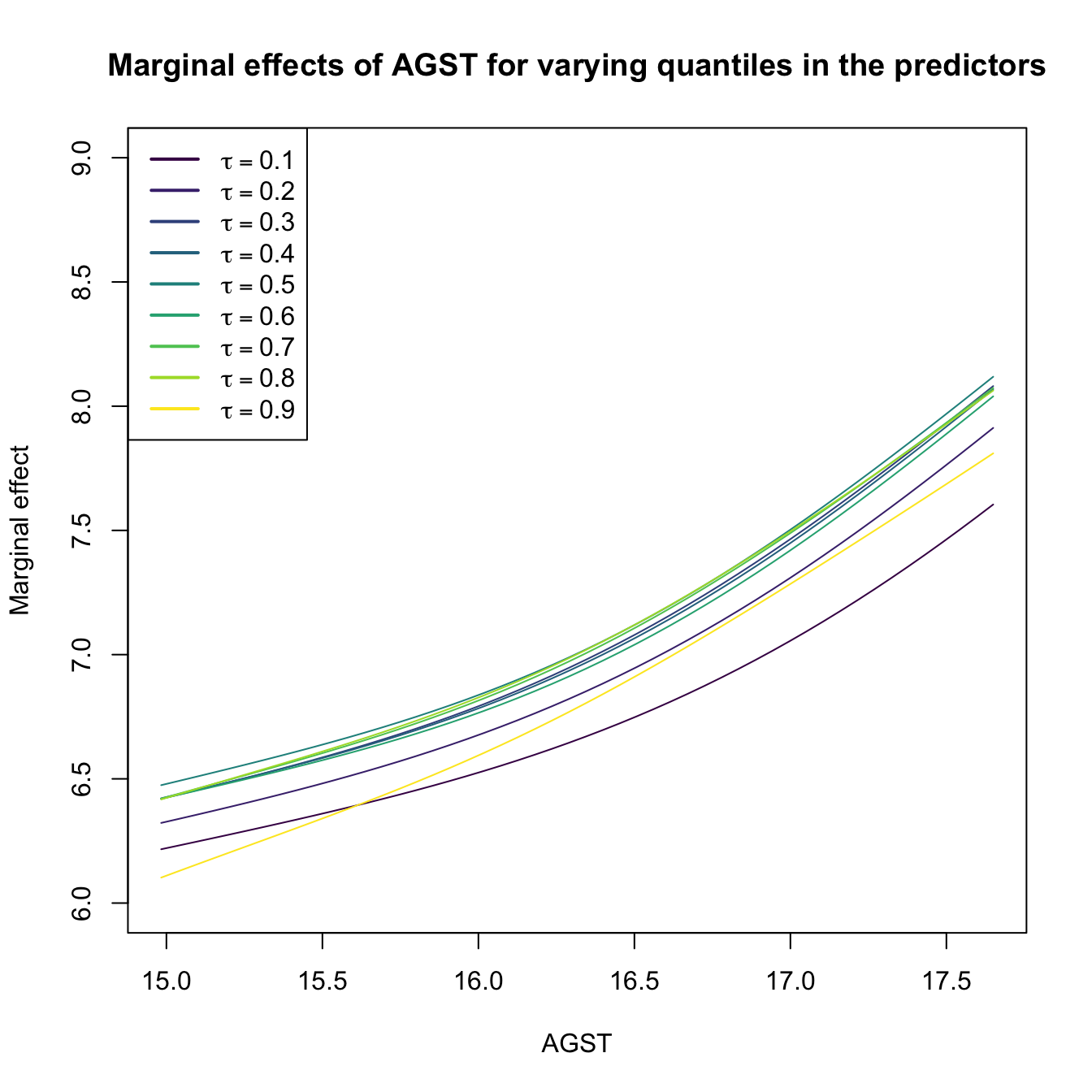


# These quantiles are
apply(wine[c("Age", "WinterRain", "HarvestRain")], 2, quantile, prob = tau)
##      Age WinterRain HarvestRain
## 10%  5.6      419.2        65.2
## 20%  8.2      508.8        86.2
## 30% 10.8      567.8        94.6
## 40% 13.4      576.2       114.4
## 50% 16.0      600.0       123.0
## 60% 18.6      609.2       156.8
## 70% 21.2      691.4       173.6
## 80% 23.8      716.4       187.0
## 90% 26.8      785.4       255.0

The summary of np::npreg returns an $R^2.$ This statistic is defined as

\[\begin{align*} R^2:=\frac{(\sum_{i=1}^n(Y_i-\bar{Y})(\hat{Y}_i-\bar{Y}))^2}{(\sum_{i=1}^n(Y_i-\bar{Y})^2)(\sum_{i=1}^n(\hat{Y}_i-\bar{Y})^2)} \end{align*}\]

and is neither the squared correlation coefficient between $Y_1,\ldots,Y_n$ and $\hat{Y}_1,\ldots,\hat{Y}_n\,$¹⁷² $\!\!^,$¹⁷³ nor “the percentage of variance explained” by the model – this interpretation makes sense within the linear model context only. It is however a quantity in $[0,1]$ that attains $R^2=1$ whenever the fit is perfect (zero variability about the curve), so it can give an idea of how explicative the estimated regression function is.

5.1.2 Kernel regression with mixed data

Non-continuous predictors can also be taken into account in nonparametric regression. The key to do so is an adequate definition of a suitable kernel function for any random variable $X,$ not just continuous. Therefore, we need to find

a positive function that is a pdf¹⁷⁴ on the support of $X$ and that allows to assign more weight to observations of the random variable that are close to a given point.

If such kernel is adequately defined, then it can be readily employed in the weights of the linear combinations that form $\hat{m}(\cdot;q,\mathbf{h}).$

We analyze next the two main possibilities for non-continuous variables:

Categorical or unordered discrete variables. For example, iris$species and Auto$origin are categorical variables in which ordering does not make any sense. Categorical variables are specified in base R by factor. Due to the lack of ordering, the basic mathematical operation behind a kernel, a distance computation¹⁷⁵, is delicate. This motivates the Aitchison and Aitken (1976) kernel.

Assume that the categorical random variable $X_d$ has $u_d$ different levels. These levels can be represented as $U_d:=\{0,1,\ldots,u_d-1\}.$ For $x_d,X_d\in U_d,$ the Aitchison and Aitken (1976) unordered discrete kernel is

\[\begin{align*} l_u(x_d,X_d;\lambda):=\begin{cases} 1-\lambda,&\text{ if }x_d=X_d,\\ \frac{\lambda}{u_d-1},&\text{ if }x_d\neq X_d, \end{cases} \end{align*}\]

where $\lambda\in[0,(u_d-1)/u_d]$ is the bandwidth. Observe that this kernel is constant if $x_d\neq X_d$: since the levels of the variable are unordered, there is no sense of proximity between them. In other words, the kernel only distinguishes if two levels are equal or not to assign weight. If $\lambda=0,$ then no weight is assigned if $x_d\neq X_d$ and no information is borrowed from different levels; hence, nonparametrically regressing $Y$ onto $X_d$ is equivalent to doing $u_d$ separate nonparametric regressions. If $\lambda=(u_d-1)/u_d,$ then all levels are assigned the same weight, regardless of $x_d;$ hence, $X_d$ is irrelevant for explaining $Y.$
Ordinal or ordered discrete variables. For example, wine$Year and Auto$cylinders are discrete variables with clear orders, but they are not continuous. These variables are specified by ordered (an ordered factor in base R). Despite the existence of an ordering, the possible distances between the observations of these variables are discrete.

Assume that the ordered discrete random variable $X_d$ takes values in a set $O_d.$ For $x_d,X_d\in O_d,$ a possible (Li and Racine 2007) ordered discrete kernel is¹⁷⁶

\[\begin{align*} l_o(x_d,X_d;\eta):=\eta^{|x_d-X_d|}, \end{align*}\]

where $\eta\in[0,1]$ is the bandwidth.¹⁷⁷ If $\eta=0,1,$ then

\[\begin{align*} l_o(x_d,X_d;0)=\begin{cases}0,&x_d\neq X_d,\\1,&x_d=X_d,\end{cases}\quad l_o(x_d,X_d;1)=1. \end{align*}\]

Hence, if $\eta=0,$ nonparametrically regressing $Y$ onto $X_d$ is equivalent to doing separate nonparametric regressions for each of the levels of $X_d.$ If $\eta=1,$ $X_d$ is irrelevant for explaining $Y.$

Exercise 5.3 Show that, for any $X_d\in U_d$ and any $\lambda\in[0,(u_d-1)/u_d],$ the kernel $x\mapsto l_u(x,X_d;\lambda)$ “integrates” one over $U_d.$

Once we have defined the suitable kernels for ordered and unordered discrete variables, we can “aggregate” information from nearby observations of mixed data. Assume that, among the $p=p_c+p_u+p_o$ predictors, the first $p_c$ are continuous, the next $p_u$ are discrete unordered (or categorical), and the last $p_o$ are discrete ordered (or ordinal). The Nadaraya–Watson for mixed multivariate data is defined as

\[\begin{align} \hat{m}(\mathbf{x};0,(\mathbf{h}_c,\boldsymbol{\lambda}_u,\boldsymbol{\eta}_o)):=\sum_{i=1}^nW^0_{i}(\mathbf{x})Y_i,\tag{5.7} \end{align}\]

with the weights of the estimator being

\[\begin{align} W^0_{i}(\mathbf{x})=\frac{L_\Pi(\mathbf{x},\mathbf{X}_i)}{\sum_{j=1}^nL_\Pi(\mathbf{x},\mathbf{X}_j)}.\tag{5.8} \end{align}\]

The weights are based on the mixed product kernel

\[\begin{align*} L_\Pi(\mathbf{x},\mathbf{X}_i):=&\,\prod_{j=1}^{p_c}K_{h_j}(x_j-X_{ij})\prod_{k=1}^{p_u}l_u(x_k,X_{ik};\lambda_k)\prod_{\ell=1}^{p_o}l_o(x_\ell,X_{i\ell};\eta_\ell), \end{align*}\]

which features the vectors of bandwidths $\mathbf{h}_c=(h_1,\ldots,h_{p_c})',$ $\boldsymbol{\lambda}_u=(\lambda_1,\ldots,\lambda_{p_u})',$ and $\boldsymbol{\eta}_o=(\eta_1,\ldots,\eta_{p_o})'$ for each cluster of equal-type predictors.

The adaptation of the local linear estimator is conceptually similar to that of the local constant, but it is more cumbersome as linear approximations make sense for quantitative variables, but not for unordered predictors. Therefore, the local linear estimator with mixed predictors is skipped in these notes.

The np package employs a variation of the previous kernels and implements the local constant and linear estimators for mixed multivariate data.

# Bandwidth by CV for local linear estimator
# Recall that Species is a factor!
bw_iris <- np::npregbw(formula = Petal.Length ~ Sepal.Width + Species,
                       data = iris)
bw_iris
## 
## Regression Data (150 observations, 2 variable(s)):
## 
##               Sepal.Width      Species
## Bandwidth(s):   0.1900717 1.093558e-08
## 
## Regression Type: Local-Constant
## Bandwidth Selection Method: Least Squares Cross-Validation
## Formula: Petal.Length ~ Sepal.Width + Species
## Bandwidth Type: Fixed
## Objective Function Value: 0.1564197 (achieved on multistart 2)
## 
## Continuous Kernel Type: Second-Order Gaussian
## No. Continuous Explanatory Vars.: 1
## 
## Unordered Categorical Kernel Type: Aitchison and Aitken
## No. Unordered Categorical Explanatory Vars.: 1
# Product kernel with 2 bandwidths

# Regression
fit_iris <- np::npreg(bw_iris)
summary(fit_iris)
## 
## Regression Data: 150 training points, in 2 variable(s)
##               Sepal.Width      Species
## Bandwidth(s):   0.1900717 1.093558e-08
## 
## Kernel Regression Estimator: Local-Constant
## Bandwidth Type: Fixed
## Residual standard error: 0.3715505
## R-squared: 0.9554132
## 
## Continuous Kernel Type: Second-Order Gaussian
## No. Continuous Explanatory Vars.: 1
## 
## Unordered Categorical Kernel Type: Aitchison and Aitken
## No. Unordered Categorical Explanatory Vars.: 1

# Plot marginal effects (for quantile 0.5) of each predictor on the response
par(mfrow = c(1, 2))
plot(fit_iris, plot.par.mfrow = FALSE)

# Options for the plot method for np::npreg can be seen at ?np::npplot

# Plot marginal effects (for quantile 0.9) of each predictor on the response
par(mfrow = c(1, 2))
plot(fit_iris, xq = 0.9, plot.par.mfrow = FALSE)

The following is an example from ?np::npreg: the modeling of the GDP growth of a country from economic indicators. The predictors contain a mix of unordered, ordered, and continuous variables.

# Load data
data(oecdpanel, package = "np")

# Bandwidth by CV for local constant -- use only two starts to reduce the
# computation time
bw_OECD <- np::npregbw(formula = growth ~ oecd + ordered(year) +
                         initgdp + popgro + inv + humancap, data = oecdpanel,
                       regtype = "lc", nmulti = 2)
bw_OECD
## 
## Regression Data (616 observations, 6 variable(s)):
## 
##                     oecd ordered(year)   initgdp     popgro      inv  humancap
## Bandwidth(s): 0.01206855     0.8794929 0.3329306 0.05972217 0.159463 0.9408607
## 
## Regression Type: Local-Constant
## Bandwidth Selection Method: Least Squares Cross-Validation
## Formula: growth ~ oecd + ordered(year) + initgdp + popgro + inv + humancap
## Bandwidth Type: Fixed
## Objective Function Value: 0.0006358702 (achieved on multistart 2)
## 
## Continuous Kernel Type: Second-Order Gaussian
## No. Continuous Explanatory Vars.: 4
## 
## Unordered Categorical Kernel Type: Aitchison and Aitken
## No. Unordered Categorical Explanatory Vars.: 1
## 
## Ordered Categorical Kernel Type: Li and Racine
## No. Ordered Categorical Explanatory Vars.: 1

# Recall that ordered(year) is doing an in-formula transformation of year,
# which is *not* codified as an ordered factor in the oecdpanel dataset
# Therefore, if ordered() was not present, year would have been treated
# as continuous, as illustrated below
np::npregbw(formula = growth ~ oecd + year + initgdp + popgro +
              inv + humancap, data = oecdpanel, regtype = "lc", nmulti = 2)
## 
## Regression Data (616 observations, 6 variable(s)):
## 
##                     oecd     year   initgdp     popgro       inv  humancap
## Bandwidth(s): 0.01644512 7.481232 0.3486883 0.05860077 0.1639842 0.8371089
## 
## Regression Type: Local-Constant
## Bandwidth Selection Method: Least Squares Cross-Validation
## Formula: growth ~ oecd + year + initgdp + popgro + inv + humancap
## Bandwidth Type: Fixed
## Objective Function Value: 0.0006338394 (achieved on multistart 1)
## 
## Continuous Kernel Type: Second-Order Gaussian
## No. Continuous Explanatory Vars.: 5
## 
## Unordered Categorical Kernel Type: Aitchison and Aitken
## No. Unordered Categorical Explanatory Vars.: 1

# A cleaner approach to avoid doing the in-formula transformation, which
# may be problematic when using predict() or np_pred_CI(), is to directly
# change in the dataset the nature of the factor/ordered variables that are
# not codified as such. For example:
oecdpanel$year <- ordered(oecdpanel$year)
bw_OECD <- np::npregbw(formula = growth ~ oecd + year + initgdp + popgro +
                         inv + humancap, data = oecdpanel,
                       regtype = "lc", nmulti = 2)
bw_OECD
## 
## Regression Data (616 observations, 6 variable(s)):
## 
##                     oecd      year   initgdp   popgro        inv humancap
## Bandwidth(s): 0.02412169 0.8945532 0.1942313 118927.8 0.09142572  1.22258
## 
## Regression Type: Local-Constant
## Bandwidth Selection Method: Least Squares Cross-Validation
## Formula: growth ~ oecd + year + initgdp + popgro + inv + humancap
## Bandwidth Type: Fixed
## Objective Function Value: 0.0006545947 (achieved on multistart 2)
## 
## Continuous Kernel Type: Second-Order Gaussian
## No. Continuous Explanatory Vars.: 4
## 
## Unordered Categorical Kernel Type: Aitchison and Aitken
## No. Unordered Categorical Explanatory Vars.: 1
## 
## Ordered Categorical Kernel Type: Li and Racine
## No. Ordered Categorical Explanatory Vars.: 1

# Regression
fit_OECD <- np::npreg(bw_OECD)
summary(fit_OECD)
## 
## Regression Data: 616 training points, in 6 variable(s)
##                     oecd      year   initgdp   popgro        inv humancap
## Bandwidth(s): 0.02412169 0.8945532 0.1942313 118927.8 0.09142572  1.22258
## 
## Kernel Regression Estimator: Local-Constant
## Bandwidth Type: Fixed
## Residual standard error: 0.01814893
## R-squared: 0.6765222
## 
## Continuous Kernel Type: Second-Order Gaussian
## No. Continuous Explanatory Vars.: 4
## 
## Unordered Categorical Kernel Type: Aitchison and Aitken
## No. Unordered Categorical Explanatory Vars.: 1
## 
## Ordered Categorical Kernel Type: Li and Racine
## No. Ordered Categorical Explanatory Vars.: 1

# Plot marginal effects of each predictor on the response
par(mfrow = c(2, 3))
plot(fit_OECD, plot.par.mfrow = FALSE)

Exercise 5.4 Obtain the local constant estimator of the regression of mpg on cylinders (ordered discrete), horsepower, weight, and origin in the data(Auto, package = "ISLR") dataset. Summarize the model and plot the marginal effects of each predictor on the response (for the quantile $0.5$).

References

Aitchison, J., and C. G. G. Aitken. 1976. “Multivariate Binary Discrimination by the Kernel Method.” Biometrika 63 (3): 413–20. https://doi.org/10.1093/biomet/63.3.413.

Li, Q., and J. S. Racine. 2007. Nonparametric Econometrics. Princeton: Princeton University Press. https://press.princeton.edu/books/hardcover/9780691121611/nonparametric-econometrics.

Here $q$ denotes the order of the polynomial fit, since $p$ stands for the number of predictors.↩︎
In particular, the consideration of Taylor expansions of $m:\mathbb{R}^p\longrightarrow\mathbb{R}$ for more than two orders that involve the vector of partial derivatives $\mathrm{D}^{\otimes s}m(\mathbf{x}),$ formed by $\frac{\partial^s m(\mathbf{x})}{\partial x_1^{s_1}\cdots \partial x_p^{s_p}},$ where $s=s_1+\cdots+s_p;$ see Section 3.1.↩︎
Observe that in the second equality we assume that $Y|\mathbf{X}=\mathbf{x}$ is continuous.↩︎
Assuming that $(\mathbf{X},Y)$ is continuous to motivate the construction of the estimator.↩︎
The fact that the kde for $(\mathbf{X},Y)$ has a product kernel between the variables $\mathbf{X}$ and $Y$ is not fundamental for constructing the Nadaraya–Watson estimator, but it simplifies the computation of the integral of the denominator of (5.2). The fact that the bandwidth matrices for estimating the $\mathbf{X}$-part of $f$ and the marginal $f_\mathbf{X}$ are equal, is fundamental to ensure an estimator for $m$ that is a weighted average (with weights adding one) of the responses $Y_1,\ldots,Y_n.$↩︎
Which increases at the order $O(p^2).$↩︎
Observe that $(X_i-x)^j$ are replaced with $(X_{ij}-x_j),$ since we only consider a linear fit and now the predictors have $p$ components.↩︎
Observe that, in an abuse of notation, we denote both the random vector $(X_1,\ldots,X_p)$ and the design matrix by $\mathbf{X}.$ However, the specific meaning of $\mathbf{X}$ should be clear from the context.↩︎
Recall that now the entries of $\hat{\boldsymbol{\beta}}_\mathbf{h}$ are estimating $\boldsymbol{\beta}=\begin{pmatrix}m(\mathbf{x})\\\mathrm{D} m(\mathbf{x})\end{pmatrix}.$ So, $\hat{\boldsymbol{\beta}}_\mathbf{h}$ gives also an estimate of the gradient $\mathrm{D} m$ evaluated at $\mathbf{x}.$↩︎
$\hat{Y}_i:=\hat{m}(\mathbf{X}_i;q,\mathbf{h}),$ $i=1,\ldots,n;$ see Section 5.3.↩︎
Because it is not guaranteed that $\bar{Y}=\bar{\hat{Y}},$ what it is required to turn $R^2$ into that squared correlation coefficient.↩︎
Although in practice it is not required for the kernel to integrate one for performing regression, as the constants of the kernels cancel out in the quotients in $\hat{m}(\cdot;q,\mathbf{h}).$↩︎
Recall $K_h(x-X_i).$↩︎
Notice that this kernel does not integrate one! To normalize it we should take the specific support of $X_d$ into account, which, e.g., could be $\{0, 1, 2, 3\}$ or $\mathbb{N}.$ This is slightly cumbersome, so we avoid it because there is no difference between normalized and unnormalized kernels for regression: the kernel normalizing constants cancel out in the computation of the weights (5.8).↩︎
Importantly, note that this kernel is assumming that the levels are equally-separated! Care is needed in applications when dealing with unequally-separated ordinal variables and using ordered with the default levels specification.↩︎