3.4 Bandwidth selection
The construction of bandwidth selectors for the multivariate kde is analogous to the univariate case. The first step is to consider the multivariate MISE
\[\begin{align*} \mathrm{MISE}[\hat{f}(\cdot;\mathbf{H})]:=&\,\mathbb{E}\left[\int (\hat{f}(\mathbf{x};\mathbf{H})-f(\mathbf{x}))^2\,\mathrm{d}\mathbf{x}\right]\\ =&\,\mathbb{E}\left[\mathrm{ISE}[\hat{f}(\cdot;\mathbf{H})]\right]\\ =&\,\int \mathrm{MSE}[\hat{f}(\mathbf{x};\mathbf{H})]\,\mathrm{d}\mathbf{x} \end{align*}\]
and define the optimal MISE bandwidth matrix as
\[\begin{align} \mathbf{H}_\mathrm{MISE}:=\arg\min_{\mathbf{H}\in\mathrm{SPD}_p}\mathrm{MISE}[\hat{f}(\cdot;\mathbf{H})],\tag{3.14} \end{align}\]
where \(\mathrm{SPD}_p\) is the set of symmetric positive definite matrices70 of size \(p.\)
In practice, obtaining (3.14) is unfeasible, and the first step towards constructing a usable selector is to derive a more practical (but close to the MISE) error criterion, such as the AMISE. The following result provides it from the bias and variance given in Theorem 3.2.
Corollary 3.1 Under A1–A3,
\[\begin{align*} \mathrm{AMISE}[\hat{f}(\cdot;\mathbf{H})]=&\,\frac{1}{4}\mu^2_2(K)R\left(\mathrm{tr}(\mathbf{H}\mathrm{H}f(\cdot))\right)+\frac{R(K)}{n|\mathbf{H}|^{1/2}}. \end{align*}\]
Therefore, \(\mathrm{AMISE}[\hat{f}(\cdot;\mathbf{H})]\to0\) when \(n\to\infty.\)
Exercise 3.8 Prove Corollary 3.1 by deriving the MSE of \(\hat{f}(\mathbf{x};\mathbf{H})\) and integrating it.
Differently to what happened in the univariate case, and despite the closed expression of the AMISE, it is not possible to obtain a general bandwidth matrix that minimizes the AMISE, that is, to obtain
\[\begin{align} \mathbf{H}_\mathrm{AMISE}:=\arg\min_{\mathbf{H}\in\mathrm{SPD}_p}\mathrm{AMISE}[\hat{f}(\cdot;\mathbf{H})]\tag{3.15} \end{align}\]
explicitly. It is possible in the special case in which \(\mathbf{H}=h^2\mathbf{I}_p,\) since \(R\left(\mathrm{tr}(\mathbf{H}\mathrm{H}f(\cdot))\right)=h^4R\left(\mathrm{tr}(\mathrm{H}f(\cdot))\right)\) and, differentiating with respect to \(h,\) it follows that
\[\begin{align} h_\mathrm{AMISE}=\left[\frac{pR(K)}{\mu_2^2(K)R\left(\mathrm{tr}(\mathrm{H}f(\cdot))\right)n}\right]^{1/(p+4)}.\tag{3.16} \end{align}\]
Exercise 3.9 Show that the expression for \(h_\mathrm{AMISE}\) minimizes \(\mathrm{AMISE}[\hat{f}(\cdot;h^2\mathbf{I}_p)].\)
Even if (3.16) has been obtained by means of a large simplification, it gives a very important insight: \(h_\mathrm{AMISE}=O(n^{-1/(p+4)}).\) Therefore, the larger the dimension \(p,\) the larger the optimal bandwidth needs to be.71 In addition, it can be seen that, for unconstrained bandwidth matrices, \(\mathbf{H}_\mathrm{AMISE}=O(n^{-2/(p+4)})\,\)72 for (3.15), so exactly the same insight holds without imposing \(\mathbf{H}=h^2\mathbf{I}_p\) for obtaining (3.16).
However, neither the computation of (3.15) (through numerical optimization over \(\mathrm{SPD}_p\)) nor of (3.16) can be performed in practice, as both depend on functionals of \(f.\)
3.4.1 Plug-in rules
The normal scale bandwidth selector, denoted by \(\hat{\mathbf{H}}_\mathrm{NS},\) escapes the dependence of the AMISE on \(f\) by replacing the latter with \(\phi_{\boldsymbol{\Sigma}}(\cdot-\boldsymbol{\mu}),\) for which the curvature term in (3.15) can be computed (using (3.10)). Conveniently, this replacement also allows us to solve explicitly (3.15) and, with the normal kernel, results in
\[\begin{align} \mathbf{H}_\mathrm{NS}=(4/(p+2))^{2/(p+4)}n^{-2/(p+4)}\boldsymbol{\Sigma}.\tag{3.17} \end{align}\]
Replacing \(\boldsymbol{\Sigma}\) by the sample covariance matrix73 \(\mathbf{S}\) in (3.17) gives \(\hat{\mathbf{H}}_\mathrm{NS},\) which can be straightforwardly computed in practice.
\(\hat{\mathbf{H}}_\mathrm{NS}\) is a zero-stage plug-in selector, a concept that was introduced in Section 2.4. The DPI selector, or henceforth simply Plug-In selector (PI), follows the same steps that were employed in Section 2.4.1 to build up an \(\ell\)-stage plug-in selector. This selector successively estimates a series of bandwidths, each of them associated with a chain of optimality problems, until “giving up” at stage \(\ell\) (usually, \(\ell=2\)) and “sweeping under the carpet” a parametric assumption for \(f\) that allows a functional of \(f\) to be estimated at the latest optimal expression. In the multivariate context, the conceptual idea is the same, but the technicalities are more demanding, with the extra nuisance of the lack of explicit expressions for the optimal bandwidths in each of the PI steps. We do not go into details74 and we just denote \(\hat{\mathbf{H}}_\mathrm{PI}\) to the bandwidth selector that extends \(\hat{h}_{\mathrm{DPI}}\) to the multivariate case.
Plug-in selectors are implemented by ks::Hns (NS), ks::Hpi (PI with full bandwidth matrix) and ks::Hpi.diag (PI with diagonal bandwidth matrix). The next chunk of code shows how to use them.
# Simulated data
n <- 500
Sigma_1 <- matrix(c(1, -0.75, -0.75, 2), nrow = 2, ncol = 2)
Sigma_2 <- matrix(c(2, -0.25, -0.25, 1), nrow = 2, ncol = 2)
set.seed(123456)
samp <- ks::rmvnorm.mixt(n = n, mus = rbind(c(2, 2), c(-2, -2)),
                         Sigmas = rbind(Sigma_1, Sigma_2),
                         props = c(0.5, 0.5))

# Normal scale bandwidth
(Hns <- ks::Hns(x = samp))
##           [,1]      [,2]
## [1,] 0.7508991 0.4587521
## [2,] 0.4587521 0.6582366

# PI bandwidth unconstrained
(Hpi <- ks::Hpi(x = samp))
##            [,1]       [,2]
## [1,] 0.26258868 0.03375926
## [2,] 0.03375926 0.23619016

# PI bandwidth diagonal
(Hpi_diag <- ks::Hpi.diag(x = samp))
##           [,1]      [,2]
## [1,] 0.2416352 0.0000000
## [2,] 0.0000000 0.2172413

# Compare kdes
par(mfrow = c(2, 2))
cont <- seq(0, 0.05, l = 20)
col <- viridis::viridis
plot(ks::kde(x = samp, H = Hns), display = "filled.contour2",
     abs.cont = cont, col.fun = col, main = "NS")
plot(ks::kde(x = samp, H = diag(diag(Hns))), display = "filled.contour2",
     abs.cont = cont, col.fun = col, main = "NS diagonal")
plot(ks::kde(x = samp, H = Hpi), display = "filled.contour2",
     abs.cont = cont, col.fun = col, main = "PI")
plot(ks::kde(x = samp, H = Hpi_diag), display = "filled.contour2",
     abs.cont = cont, col.fun = col, main = "PI diagonal")
Density derivative estimation
The normal scale selector expands in a simple fashion to the problem of selecting the optimal bandwidth for estimating the \(r\)-th derivative of \(f.\) The solution to this problem follows a path completely parallel to the density case. To begin with, the MISE of the density derivative estimator \(\widehat{\mathrm{D}^{\otimes r}f}(\cdot;\mathbf{H})\) is defined as75
\[\begin{align*} \mathrm{MISE}[\widehat{\mathrm{D}^{\otimes r}f}(\cdot;\mathbf{H})]:=\mathbb{E}\left[\int \|\widehat{\mathrm{D}^{\otimes r}f}(\mathbf{x};\mathbf{H})-\mathrm{D}^{\otimes r}f(\mathbf{x})\|^2\,\mathrm{d}\mathbf{x}\right]. \end{align*}\]
After obtaining an explicit form for \(\mathrm{AMISE}[\widehat{\mathrm{D}^{\otimes r}f}(\cdot;\mathbf{H})],\) the assumption that \(f=\phi_{\boldsymbol{\Sigma}}(\cdot-\boldsymbol{\mu})\) for computing the functional depending on \(f,\) and the use of the normal kernel, the normal scale bandwidth selector for the \(r\)-th derivative of \(f\) follows:
\[\begin{align} \mathbf{H}_{\mathrm{NS},r}=(4/(p+2r+2))^{2/(p+2r+4)}n^{-2/(p+2r+4)}\boldsymbol{\Sigma}.\tag{3.18} \end{align}\]
Replacing \(\boldsymbol{\Sigma}\) by the sample covariance matrix \(\mathbf{S}\) in (3.18) gives \(\hat{\mathbf{H}}_{\mathrm{NS},r},\) which is remarkably simple to compute in practice.
Observe that \(\mathbf{H}_{\mathrm{NS},0}=\mathbf{H}_{\mathrm{NS}}\) and that the factor \(f_{n,p,r}:=(4/(p+2r+2))^{2/(p+2r+4)}n^{-2/(p+2r+4)}\) increases as \(r\) increases (see Figure 3.3), indicating that optimal bandwidths for derivative estimation are larger than optimal bandwidths for density estimation (\(r=0\)). Indeed, it can be seen that \(\mathbf{H}_{\mathrm{AMISE},r}=O(n^{-2/(p+2r+4)}).\) Therefore, employing an optimal bandwidth for density estimation to estimate a derivative will result in an undersmoothing of the derivative.
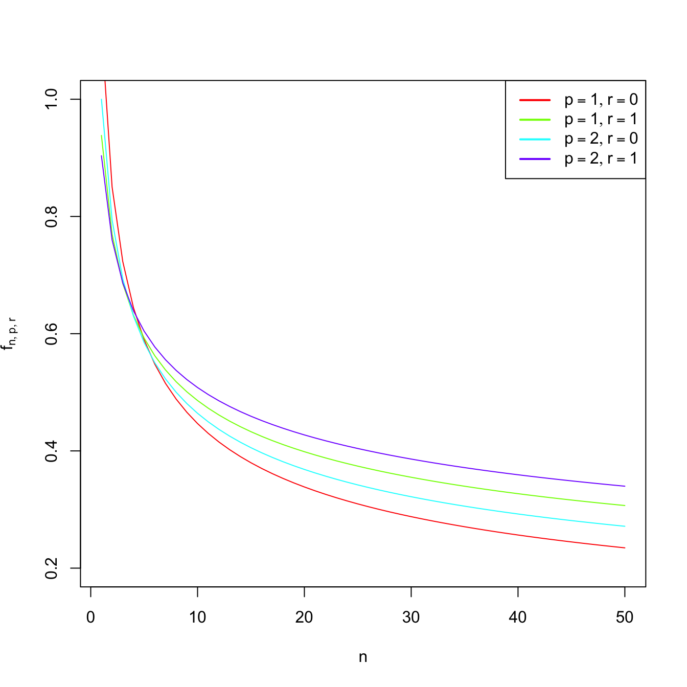
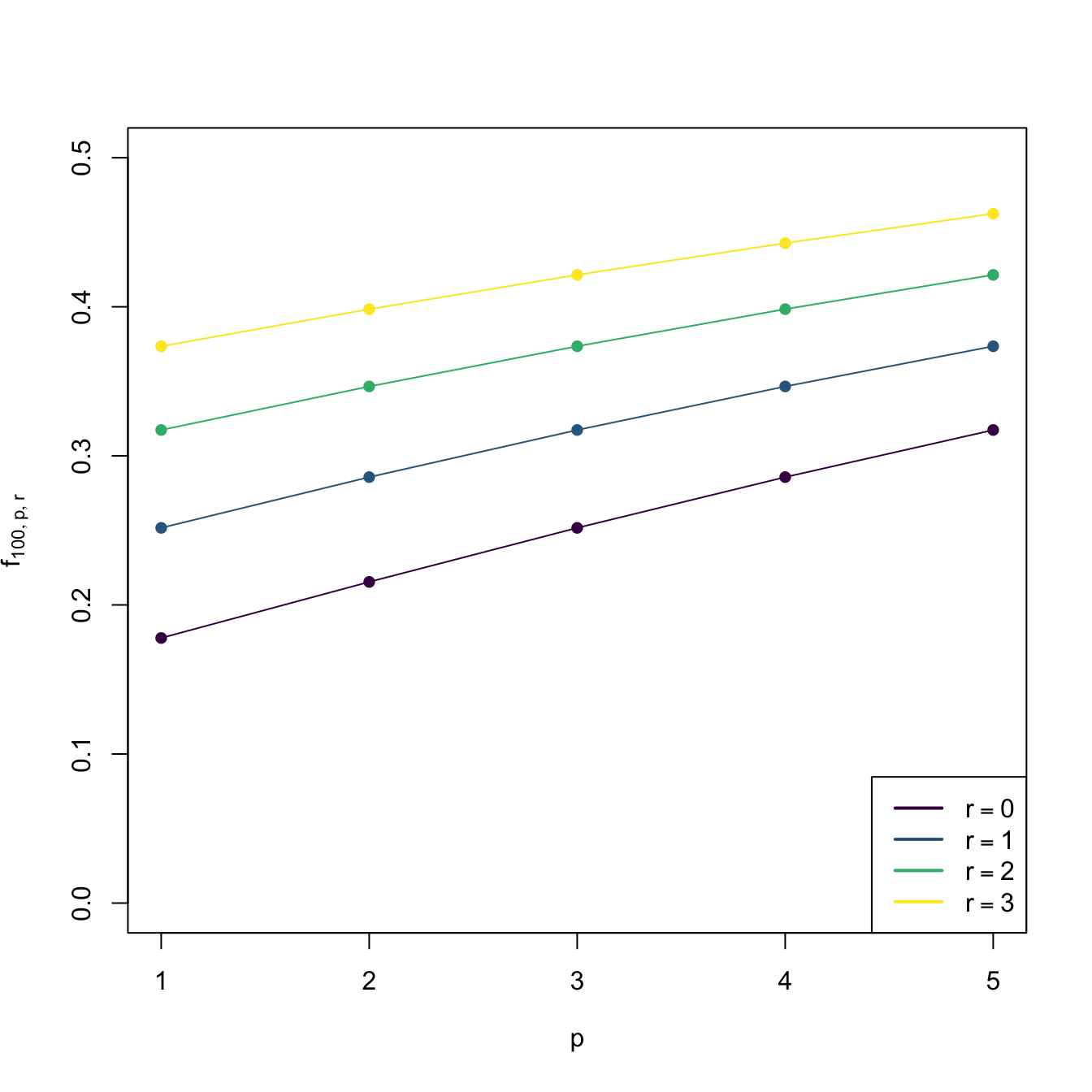
Figure 3.3: Graphs of \(n\mapsto f_{n,p,r}\) (for varying \(p\) and \(r\)) and \(p\mapsto f_{n,p,r}\) (for \(n=100\) and varying \(r\)).
The PI selector also admits a derivative version, \(\hat{\mathbf{H}}_{\mathrm{PI},r},\) which sacrifices the simplicity of (3.18) to gain performance on estimating \(\mathbf{H}_{\mathrm{AMISE},r}\) for non-normal-like densities.
# Normal scale bandwidth (compare with Hns)
(Hns1 <- ks::Hns(x = samp, deriv.order = 1))
##          [,1]      [,2]
## [1,] 1.138867 0.6957760
## [2,] 0.695776 0.9983282

# PI bandwidth unconstrained (compare with Hpi)
(Hpi1 <- ks::Hpi(x = samp, deriv.order = 1))
##           [,1]      [,2]
## [1,] 0.3248011 0.1125982
## [2,] 0.1125982 0.3017212

# PI bandwidth diagonal (compare with Hpi_diag)
(Hpi_diag1 <- ks::Hpi.diag(x = samp, deriv.order = 1))
##           [,1]      [,2]
## [1,] 0.2854801 0.0000000
## [2,] 0.0000000 0.2545556

# Compare kddes
par(mfrow = c(2, 2))
cont <- seq(-0.02, 0.02, l = 21)
plot(ks::kdde(x = samp, H = Hns1, deriv.order = 1),
     display = "filled.contour2", main = "NS", abs.cont = cont)
plot(ks::kdde(x = samp, H = diag(diag(Hns1)), deriv.order = 1),
     display = "filled.contour2", main = "NS diagonal", abs.cont = cont)
plot(ks::kdde(x = samp, H = Hpi1, deriv.order = 1),
     display = "filled.contour2", main = "PI", abs.cont = cont)
plot(ks::kdde(x = samp, H = Hpi_diag1, deriv.order = 1),
     display = "filled.contour2", main = "PI diagonal", abs.cont = cont)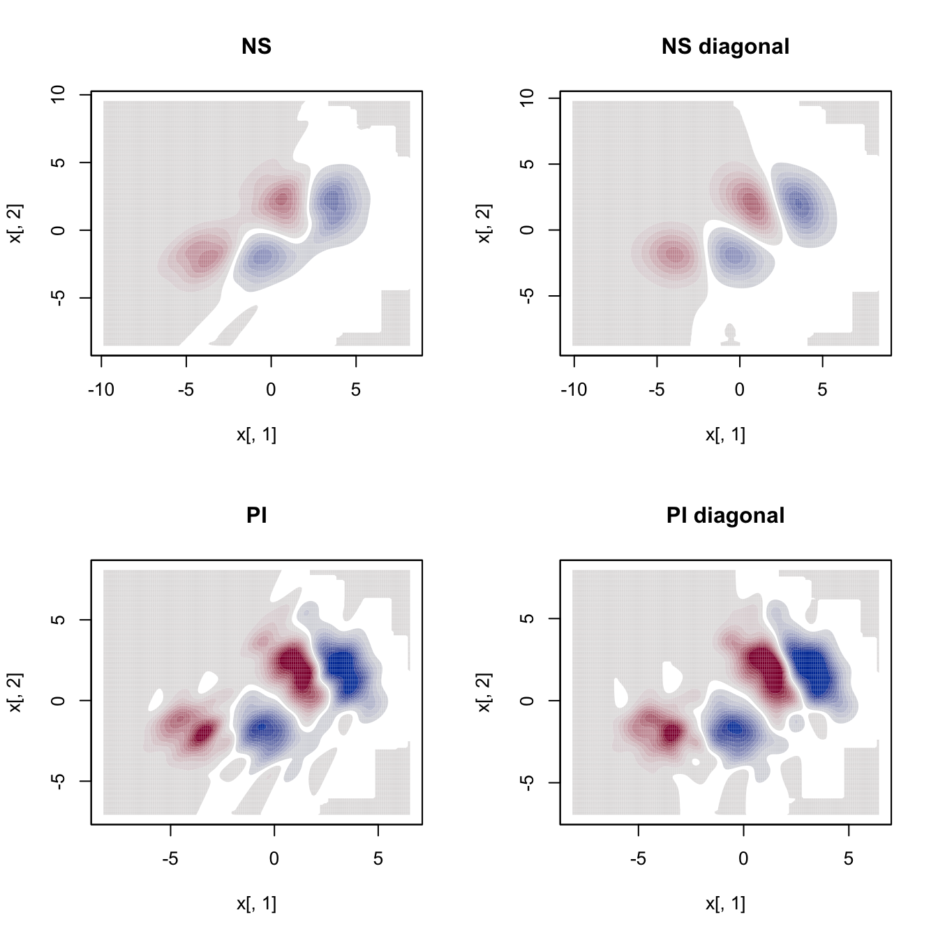
Exercise 3.10 The data(sunspots_births, package = "rotasym") dataset contains the recorded sunspots births during 1872–2018 from the Debrecen Photoheliographic Data (DPD) catalog. The dataset presents \(51,303\) sunspot records, featuring their positions in spherical coordinates (theta and phi), sizes (total_area), and distances to the center of the solar disk (dist_sun_disc).
- Compute and plot the kde for
phiusing the DPI selector. Describe the result. - Compute and plot the kernel density derivative estimator for
phiusing the adequate DPI selector. Determine approximately the location of the main mode(s). - Compute the log-transformed kde with
adj.positive = 1fortotal_areausing the NS selector. - Draw the histogram of \(M=10,000\) samples simulated from the kde obtained in a.
3.4.2 Cross-validation
The Least Squares Cross-Validation (LSCV) selector directly extends from the univariate case and attempts to minimize \(\mathrm{MISE}[\hat{f}(\cdot;\mathbf{H})]\) by estimating it unbiasedly with
\[\begin{align*} \mathrm{LSCV}(\mathbf{H}):=\int\hat{f}(\mathbf{x};\mathbf{H})^2\,\mathrm{d}\mathbf{x}-2n^{-1}\sum_{i=1}^n\hat{f}_{-i}(\mathbf{X}_i;\mathbf{H}) \end{align*}\]
and then minimizing that loss:
\[\begin{align*} \hat{\mathbf{H}}_\mathrm{LSCV}:=\arg\min_{\mathbf{H}\in\mathrm{SPD}_p}\mathrm{LSCV}(\mathbf{H}). \end{align*}\]
Biased Cross-Validation (BCV) combines the cross-validation ideas from \(\hat{\mathbf{H}}_\mathrm{LSCV}\) with the plug-in ideas behind \(\hat{\mathbf{H}}_\mathrm{PI}\) to build, in a way analogous to the univariate case (see (2.30)), the \(\hat{\mathbf{H}}_\mathrm{BCV}\) selector. This selector trades the unbiasedness of \(\hat{\mathbf{H}}_\mathrm{LSCV}\) for a reduction in its variance.
Cross-validatory selectors, allowing for full or diagonal bandwidth matrices, are implemented by ks::Hlscv and ks::Hlscv.diag (LSCV), and ks::Hbcv and ks::Hbcv.diag (BCV). The following chunk of code shows how to use them.
# LSCV bandwidth unconstrained
Hlscv <- ks::Hlscv(x = samp)

# LSCV bandwidth diagonal
Hlscv_diag <- ks::Hlscv.diag(x = samp)

# BCV bandwidth unconstrained
Hbcv <- ks::Hbcv(x = samp)

# BCV bandwidth diagonal
Hbcv_diag <- ks::Hbcv.diag(x = samp)

# Compare kdes
par(mfrow = c(2, 2))
cont <- seq(0, 0.03, l = 20)
col <- viridis::viridis
plot(ks::kde(x = samp, H = Hlscv), display = "filled.contour2",
     abs.cont = cont, col.fun = col, main = "LSCV")
plot(ks::kde(x = samp, H = Hlscv_diag), display = "filled.contour2",
     abs.cont = cont, col.fun = col, main = "LSCV diagonal")
plot(ks::kde(x = samp, H = Hbcv), display = "filled.contour2",
     abs.cont = cont, col.fun = col, main = "BCV")
plot(ks::kde(x = samp, H = Hbcv_diag), display = "filled.contour2",
     abs.cont = cont, col.fun = col, main = "BCV diagonal")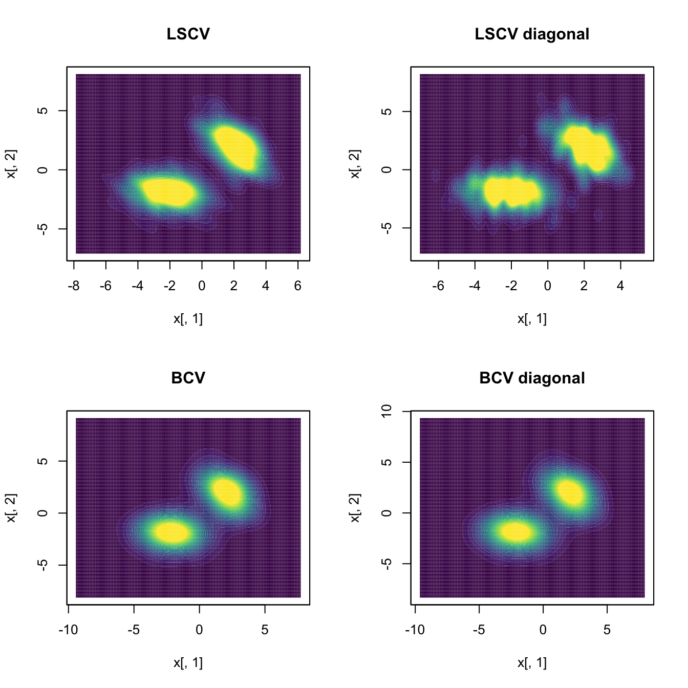
Exercise 3.11 Consider the normal mixture
\[\begin{align*} w\mathcal{N}_2(\boldsymbol{\mu}_1,\boldsymbol{\Sigma}_1)+(1 - w)\mathcal{N}_2(\boldsymbol{\mu}_2,\boldsymbol{\Sigma}_2), \end{align*}\]
where \(w=0.3,\) \(\boldsymbol{\mu}_1=(1, 1)',\) \(\boldsymbol{\mu}_2=(-1, -1)',\) \(\boldsymbol{\Sigma}_i=\begin{pmatrix}\sigma^2_{i1}&\sigma_{i1}\sigma_{i2}\rho_i\\\sigma_{i1}\sigma_{i2}\rho_i&\sigma_{i2}^2\end{pmatrix},\) \(i=1,2,\) and \(\sigma_{11}^2=\sigma_{21}^2=1,\) \(\sigma_{12}^2=\sigma_{22}^2=2,\) \(\rho_1=0.5,\) and \(\rho_2=-0.5.\)
Perform the following simulation exercise:
- Plot the density of the mixture using
ks::dmvnorm.mixtand overlay points simulated employingks::rmvnorm.mixt. You may want to useks::contourLevelsto produce density plots comparable to the kde plots performed in the next step. - Compute the kde employing \(\hat{\mathbf{H}}_{\mathrm{PI}},\) both for full and diagonal bandwidth matrices. Are there any gains on considering full bandwidths? What if \(\rho_2=0.7\)?
- Consider the previous point with \(\hat{\mathbf{H}}_{\mathrm{LSCV}}\) instead of \(\hat{\mathbf{H}}_{\mathrm{PI}}.\) Are the conclusions the same?
References
Observe that implementing the optimization of (3.14) is not trivial, since it is required to enforce the constrain \(\mathbf{H}\in\mathrm{SPD}_p.\) A neat way of parametrizing \(\mathbf{H}\) that induces the positive definiteness constrain is through the (unique) Cholesky decomposition of \(\mathbf{H}\in\mathrm{SPD}_p\): \(\mathbf{H}=\mathbf{R}'\mathbf{R},\) where \(\mathbf{R}\) is a triangular matrix with positive entries on the diagonal (but the remaining entries unconstrained). Therefore, optimization of (3.14) (if \(f\) was known) can be done through the \(\frac{p(p+1)}{2}\) entries of \(\mathbf{R}.\)↩︎
Intuitively, this fact can be regarded as the necessity of \(h_\mathrm{AMISE}\) to account for larger neighborhoods about \(\mathbf{x},\) as the emptiness of the space \(\mathbb{R}^p\) grows with \(p.\)↩︎
Recall that, restricting to specific bandwidths like \(\mathbf{H}=h^2\mathbf{I}_p,\) then \(\mathbf{H}_\mathrm{AMISE}=h_\mathrm{AMISE}^2\mathbf{I}_p,\) so the expressions \(h_\mathrm{AMISE}=O(n^{-1/(p+4)})\) and \(\mathbf{H}_\mathrm{AMISE}=O(n^{-2/(p+4)})\) are perfectly coherent.↩︎
Or by a robust estimator of \(\boldsymbol{\Sigma}.\)↩︎
The interested reader is referred to Section 3.6 in Chacón and Duong (2018) for an excellent exposition.↩︎
Note the presence of the squared norm \(\|\cdot\|^2\) in the integrand, as \(\widehat{\mathrm{D}^{\otimes r}f}(\mathbf{x};\mathbf{H})-\mathrm{D}^{\otimes r}f(\mathbf{x})\) is a vector in \(\mathbb{R}^{p^r}.\)↩︎