3.2 Density derivative estimation

As we will see in Section 3.5, sometimes it is interesting to estimate the derivatives of the density, particularly the gradient and the Hessian, rather than the density itself.

For a density $f:\mathbb{R}^p\longrightarrow\mathbb{R}$ its gradient $\mathrm{D}f:\mathbb{R}^p\longrightarrow\mathbb{R}^p$ is defined as

\[\begin{align*} \mathrm{D}f(\mathbf{x}):=\begin{pmatrix}\frac{\partial f(\mathbf{x})}{\partial x_1}\\\vdots\\\frac{\partial f(\mathbf{x})}{\partial x_p}\end{pmatrix}, \end{align*}\]

which can be regarded as the result of applying the differential operator $\mathrm{D}:=\left(\frac{\partial }{\partial x_1},\ldots,\frac{\partial}{\partial x_p}\right)'$ to $f.$ The Hessian of $f$ is the matrix

\[\begin{align*} \mathrm{H}f(\mathbf{x}):=\left(\frac{\partial^2 f(\mathbf{x})}{\partial x_i\partial x_j}\right),\quad i,j=1,\ldots,p. \end{align*}\]

The Hessian is a well-known object in multivariate calculus, but in the way it is defined somehow closes the way to the construction of high-order derivatives that admit a simple algebraic disposition.⁵³ Thus, an alternative arrangement of the Hessian is imperative, and this can by achieved by its columnwise stacking performed by the $\mathrm{vec}$ operator. The $\mathrm{vec}$ operator stacks the columns of any matrix into a long vector⁵⁴ and makes the Hessian operator $\mathrm{H}:=\left(\frac{\partial^2 }{\partial x_i\partial x_j}\right)$ expressible as the vector

\[\begin{align} \mathrm{vec}\,\mathrm{H}=\begin{pmatrix}\frac{\partial^2}{\partial x_1\partial x_1}\\\vdots\\\frac{\partial^2}{\partial x_p\partial x_p}\end{pmatrix}\in\mathbb{R}^{p^2}.\tag{3.3} \end{align}\]

Interestingly, (3.3) coincides with the Kronecker product⁵⁵ of $\mathrm{D}$ with itself: $\mathrm{D}^{\otimes 2}:=\mathrm{D}\otimes\mathrm{D}$ (a column vector with $p^2$ entries). That is,

\[\begin{align} \mathrm{vec}(\mathrm{H}f(\mathbf{x}))=\mathrm{D}^{\otimes 2}f(\mathbf{x}).\tag{3.4} \end{align}\]

The previous relation may seem to be just a mathematical formalism without a clear practical relevance. However, it is key for simplifying the consideration of second and high-order derivatives of a function $f.$ Indeed, the $r$-th derivatives of $f,$ for $r\geq 0\,$⁵⁶, can now be collected in terms of the $r$-fold Kronecker product of $\mathrm{D}$:

\[\begin{align} \mathrm{D}^{\otimes r}f(\mathbf{x}):=\begin{pmatrix} \frac{\partial^rf(\mathbf{x})}{\partial x_1\cdots\partial x_1}\\ \vdots\\ \frac{\partial^rf(\mathbf{x})}{\partial x_1\cdots\partial x_p}\\ \vdots\\ \frac{\partial^rf(\mathbf{x})}{\partial x_p\cdots\partial x_p}\end{pmatrix}\in\mathbb{R}^{p^r}.\tag{3.5} \end{align}\]

This formalism is extremely useful, for example, to obtain a compact expansion of the univariate Taylor’s theorem (Theorem 1.11).

Theorem 3.1 (Multivariate Taylor's Theorem) Let $f:\mathbb{R}^p\longrightarrow\mathbb{R}$ and $\mathbf{x}\in\mathbb{R}^p.$ Assume that $f$ has $r$ continuous derivatives in $B(\mathbf{x},\delta):=\{\mathbf{y}\in\mathbb{R}^p: \|\mathbf{y}-\mathbf{x}\|<\delta\}.$ Then, for any $\|\mathbf{h}\|<\delta,$

\[\begin{align} f(\mathbf{x}+\mathbf{h})=\sum_{j=0}^r\frac{1}{j!}(\mathrm{D}^{\otimes j}f(\mathbf{x}))'\mathbf{h}^{\otimes j}+R_r,\quad R_r=o(\|\mathbf{h}\|^r).\tag{3.6} \end{align}\]

Observe the compactness and scalability of (3.6), featuring multiplications between vectors of lengths $p^j$ for $j=0,\ldots,r.$ This contrasts with the traditional second-order⁵⁷ multivariate Taylor expansion:

\[\begin{align*} f(\mathbf{x}+\mathbf{h})=f(\mathbf{x})+(\mathrm{D}f(\mathbf{x}))'\mathbf{h}+\frac{1}{2}\mathbf{h}'\mathrm{H}f(\mathbf{x})\mathbf{h}+o(\|\mathbf{h}\|^2). \end{align*}\]

Exercise 3.2 Let $f(x,y):=x^3+\cos(y).$ Compute:

$\mathrm{D}f$ and $\mathrm{H}f.$
$\mathrm{D}^{\otimes 2}f.$ Check that $\mathrm{vec}(\mathrm{H}f)=\mathrm{D}^{\otimes 2}f.$
$\mathrm{D}^{\otimes 3}f=\mathrm{D}\otimes\mathrm{D}^{\otimes 2}f.$
The Taylor expansion of $f$ at $\mathbf{x}=(1,0)'$ for the first, second, and third orders.

Exercise 3.3 Considering the setting in Exercise 3.2:

Plot the surface for $f$ about $\mathbf{x}=(1,0)'.$
Plot the surfaces for the three Taylor expansions at $\mathbf{x}=(1,0)'$ and verify their increasing accuracy on approximating $f.$

For visualizing the different surfaces, rely on several image panels with the same vertical scale or use rgl::surface3d.

Exercise 3.4 Perform Exercises 3.2 and 3.3 using the function $f(x,y)=\phi_{\sigma_1}(x)\phi_{\sigma_2}(y)$ and $\mathbf{x}=(0,0)'.$ Consider $\sigma_1=\sigma_2=1,$ and $\sigma_1=1.25$ and $\sigma_2=0.75.$

Employing the (3.5) operator, the kernel estimator for the $r$-th derivative⁵⁸ $\mathrm{D}^{\otimes r}f$ is defined as the application of the operator $\mathrm{D}^{\otimes r}$ to the kde $\hat{f}(\cdot;\mathbf{H})$:

\[\begin{align} \widehat{\mathrm{D}^{\otimes r}f}(\mathbf{x};\mathbf{H}):=\mathrm{D}^{\otimes r}\hat{f}(\mathbf{x};\mathbf{H})=\frac{1}{n}\sum_{i=1}^n(\mathrm{D}^{\otimes r}K_{\mathbf{H}})(\mathbf{x}-\mathbf{X}_i),\tag{3.7} \end{align}\]

where $\mathrm{D}^{\otimes r}K_{\mathbf{H}}$ can be computed as

\[\begin{align} \mathrm{D}^{\otimes r}K_{\mathbf{H}}=|\mathbf{H}|^{-1/2}(\mathbf{H}^{-1/2})^{\otimes r}(\mathrm{D}^{\otimes r}K)(\mathbf{H}^{-1/2}(\mathbf{x}-\mathbf{X}_i)).\tag{3.8} \end{align}\]

The gradient estimator has a key relevance in Section 3.5.2 and is the simplest derivative estimator. Its form follows either by replacing $r=1$ in (3.7) and (3.8) or by directly differentiating (3.1):

\[\begin{align*} \widehat{\mathrm{D}f}(\mathbf{x};\mathbf{H})=\frac{\mathbf{H}^{-1/2}}{n|\mathbf{H}|^{1/2}}\sum_{i=1}^n(\mathrm{D}K)(\mathbf{H}^{-1/2}(\mathbf{x}-\mathbf{X}_i)). \end{align*}\]

If we set $(\mathrm{D}K)_{\mathbf{H}}(\mathbf{x}-\mathbf{X}_i):=|\mathbf{H}|^{-1/2}(\mathrm{D}K)(\mathbf{H}^{-1/2}(\mathbf{x}-\mathbf{X}_i)),$ then it can clearly be seen that

\[\begin{align*} \widehat{\mathrm{D}f}(\mathbf{x};\mathbf{H})=\frac{\mathbf{H}^{-1/2}}{n}\sum_{i=1}^n(\mathrm{D}K)_{\mathbf{H}}(\mathbf{x}-\mathbf{X}_i) \end{align*}\]

and how the extra factor $\mathbf{H}^{-1/2}$ appears. This extra factor explains why the optimal bandwidth selectors for (3.1) and (3.7) are different. The estimator of the Hessian will be employed in Section 3.5.4.

The estimator (3.7) can be computed using ks::kdde. The following code presents how to do so for $p=1$ and $r=1,2.$

# Simulated univariate data
n <- 1e3
set.seed(324178)
x <- nor1mix::rnorMix(n = n, obj = nor1mix::MW.nm8)

# Location of relative extrema
dens <- function(x) nor1mix::dnorMix(x, obj = nor1mix::MW.nm8)
minus_dens <- function(x) -dens(x)
extrema <- c(nlm(f = minus_dens, p = 0)$estimate,
             nlm(f = dens, p = 0.75)$estimate,
             nlm(f = minus_dens, p = 1.5)$estimate)

# Plot target density
par(mfrow = c(2, 2))
plot(nor1mix::MW.nm8, p.norm = FALSE)
rug(x)
abline(v = extrema, col = c(3, 2, 3))

# Density estimation (automatically chosen bandwidth)
kdde_0 <- ks::kdde(x = x, deriv.order = 0)
plot(kdde_0, xlab = "x", main = "Density estimation")
abline(v = extrema, col = c(3, 2, 3))

# Density derivative estimation (automatically chosen bandwidth, but different
# from kdde_0!)
kdde_1 <- ks::kdde(x = x, deriv.order = 1)
plot(kdde_1, xlab = "x", main = "Density derivative estimation")
abline(v = extrema, col = c(3, 2, 3))

# Density second derivative estimation
kdde_2 <- ks::kdde(x = x, deriv.order = 2)
plot(kdde_2, xlab = "x", main = "Density second derivative estimation")
abline(v = extrema, col = c(3, 2, 3))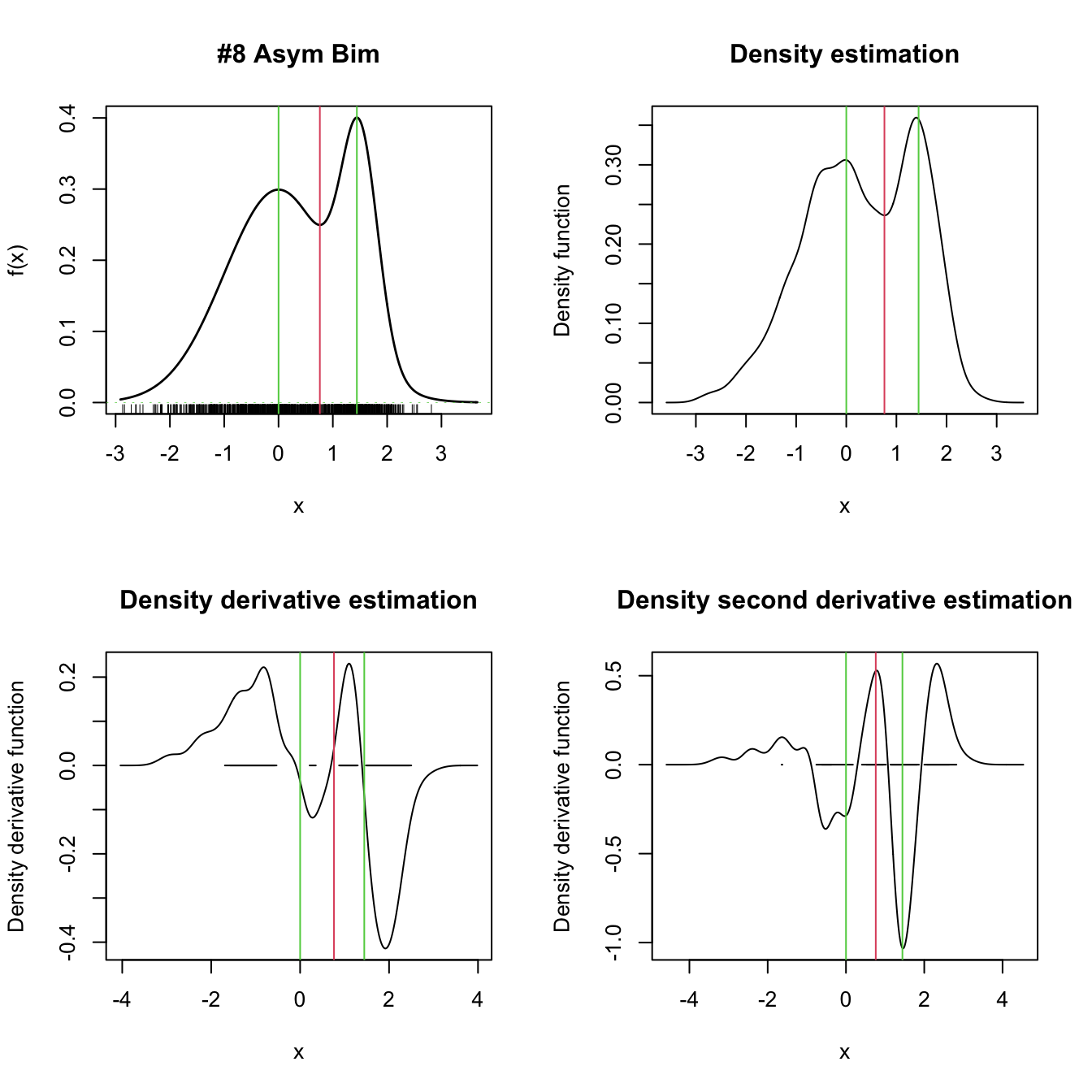

$Univariate density derivative estimation for $r=0,1,2.$ The green vertical bars represent the modes (local maxima) and the red vertical bar the antimode (local minimum) of nor1mix::MW8. Observe how the density derivative estimation vanishes at the local extrema and how the second derivative estimation captures the sign of the extrema, thus indicating the presence of a mode or an antimode.$

Figure 3.2: Univariate density derivative estimation for $r=0,1,2.$ The green vertical bars represent the modes (local maxima) and the red vertical bar the antimode (local minimum) of nor1mix::MW8. Observe how the density derivative estimation vanishes at the local extrema and how the second derivative estimation captures the sign of the extrema, thus indicating the presence of a mode or an antimode.

The following code presents how to do so for $p=2$ and $r=1,2.$

# Simulated bivariate data
n <- 1e3
mu_1 <- rep(1, 2)
mu_2 <- rep(-1.5, 2)
Sigma_1 <- matrix(c(1, -0.75, -0.75, 3), nrow = 2, ncol = 2)
Sigma_2 <- matrix(c(2, 0.75, 0.75, 3), nrow = 2, ncol = 2)
w <- 0.45
set.seed(324178)
x <- ks::rmvnorm.mixt(n = n, mus = rbind(mu_1, mu_2),
                      Sigmas = rbind(Sigma_1, Sigma_2), props = c(w, 1 - w))

# Density estimation
kdde_0 <- ks::kdde(x = x, deriv.order = 0)
plot(kdde_0, display = "filled.contour2", xlab = "x", ylab = "y")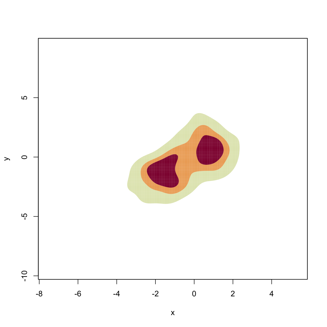


# Density derivative estimation
kdde_1 <- ks::kdde(x = x, deriv.order = 1)
str(kdde_1$estimate)
## List of 2
##  $ : num [1:151, 1:151] -4.76e-19 4.18e-19 1.18e-19 -6.27e-20 -3.74e-19 ...
##  $ : num [1:151, 1:151] -7.66e-19 -1.18e-18 -4.19e-19 -6.70e-19 -8.30e-19 ...
# $estimate is now a list of two matrices with each of the derivatives

# Plot of the gradient field - arrows pointing towards the modes
plot(kdde_1, display = "quiver", xlab = "x", ylab = "y")


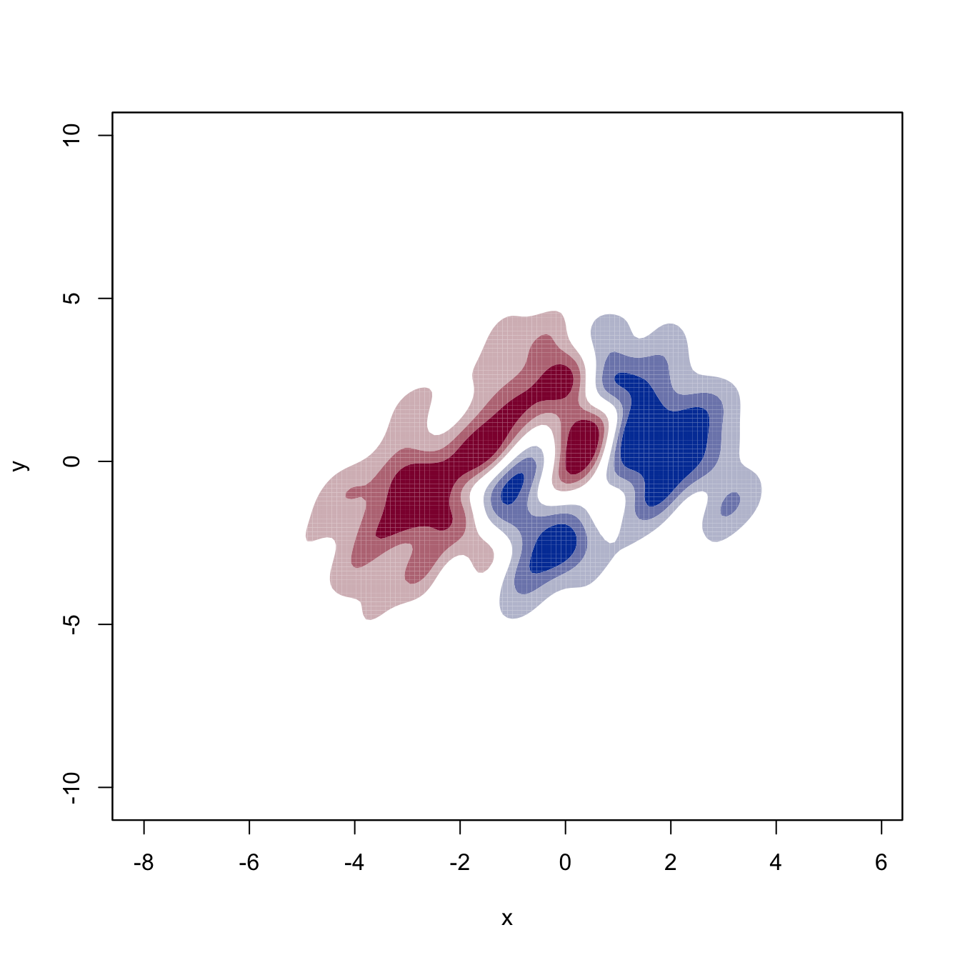
# Plot of the two components of the gradient field
for(i in 1:2) {
  plot(kdde_1, display = "filled.contour2", which.deriv.ind = i,
       xlab = "x", ylab = "y")
}


# Second density derivative estimation
kdde_2 <- ks::kdde(x = x, deriv.order = 2)
str(kdde_2$estimate)
## List of 4
##  $ : num [1:151, 1:151] -2.53e-19 -6.84e-19 -2.33e-19 -1.33e-18 -4.44e-19 ...
##  $ : num [1:151, 1:151] -1.55e-20 9.60e-20 3.56e-19 7.44e-20 1.11e-19 ...
##  $ : num [1:151, 1:151] -1.55e-20 9.60e-20 3.56e-19 7.44e-20 1.11e-19 ...
##  $ : num [1:151, 1:151] -5.53e-19 -3.68e-19 6.63e-21 -7.58e-19 -1.28e-19 ...
# $estimate is now a list of four matrices with each of the derivatives

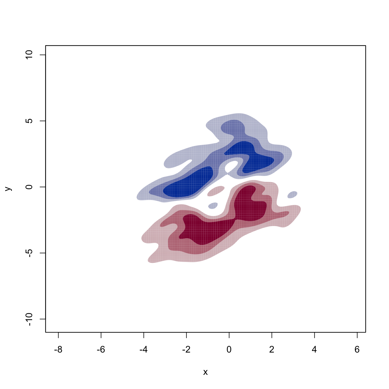
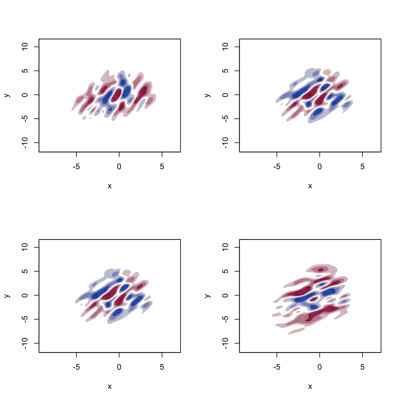
# Plot of the two components of the gradient field ("which.deriv.ind" indicates
# the index in the Kronecker product)
par(mfcol = c(2, 2))
for(i in 1:4) {
  plot(kdde_2, display = "filled.contour2", which.deriv.ind = i,
       xlab = "x", ylab = "y")
}

Exercise 3.5 Inspecting the second derivatives of a bivariate kde can be challenging. For that reason, the summary curvature $s(\mathbf{x})=-1_{\{\mathrm{H}f(\mathbf{x})\text{ is negative definite}\}}||\mathrm{H}f(\mathbf{x})||$ is often considered, as it serves for indicating the presence and “strength” of a local mode. Implement, from the output of ks::kdde, the kernel estimator for $s.$ Then, compare your implementation with the function ks::kcurv and use both to determine the presence of modes in the previous example.

To evaluate the performance of kernel estimators of the derivatives, it is very useful to recall that the gradient and Hessian of a multivariate normal density $\phi_{\boldsymbol{\Sigma}}(\cdot-\boldsymbol{\mu})$ are:⁵⁹

\[\begin{align} \mathrm{D}\phi_{\boldsymbol{\Sigma}}(\mathbf{x}-\boldsymbol{\mu})&=-\phi_{\boldsymbol{\Sigma}}(\mathbf{x}-\boldsymbol{\mu})\boldsymbol{\Sigma}^{-1}(\mathbf{x}-\boldsymbol{\mu}),\tag{3.9}\\ \mathrm{H}\phi_{\boldsymbol{\Sigma}}(\mathbf{x}-\boldsymbol{\mu})&=\phi_{\boldsymbol{\Sigma}}(\mathbf{x}-\boldsymbol{\mu})\boldsymbol{\Sigma}^{-1}\left((\mathbf{x}-\boldsymbol{\mu})(\mathbf{x}-\boldsymbol{\mu})'-\boldsymbol{\Sigma}\right)\boldsymbol{\Sigma}^{-1}.\tag{3.10} \end{align}\]

These functions can be implemented as follows.

# Gradient of a N(mu, Sigma) density (vectorized on x)
grad_norm <- function(x, mu, Sigma) {

  # Check dimensions
  x <- rbind(x)
  p <- length(mu)
  stopifnot(ncol(x) == p & nrow(Sigma) == p & ncol(Sigma) == p)

  # Gradient
  grad <- -mvtnorm::dmvnorm(x = x, mean = mu, sigma = Sigma) *
    t(t(x) - mu) %*% solve(Sigma)
  return(grad)

}

# Hessian of a N(mu, Sigma) density (vectorized on x)
Hess_norm <- function(x, mu, Sigma) {

  # Check dimensions
  x <- rbind(x)
  p <- length(mu)
  stopifnot(ncol(x) == p & nrow(Sigma) == p & ncol(Sigma) == p)

  # Hessian
  Sigma_inv <- solve(Sigma)
  H <- apply(x, 1, function(y) {
    mvtnorm::dmvnorm(x = y, mean = mu, sigma = Sigma) *
      (Sigma_inv %*% tcrossprod(y - mu) %*% Sigma_inv - Sigma_inv)
  })

  # As an array
  return(array(data = c(H), dim = c(p, p, nrow(x))))

}

Obviously, in the case of a mixture $\sum_{j=1}^rw_j\phi_{\boldsymbol{\Sigma}_j}(\mathbf{x}-\boldsymbol{\mu}_j),$ the gradient becomes $\sum_{j=1}^rw_j\mathrm{D}\phi_{\boldsymbol{\Sigma}_j}(\mathbf{x}-\boldsymbol{\mu}_j)$ and the Hessian, $\sum_{j=1}^rw_j\mathrm{H}\phi_{\boldsymbol{\Sigma}_j}(\mathbf{x}-\boldsymbol{\mu}_j).$

Exercise 3.6 Graphically evaluate the accuracy on estimating the density gradient and Hessian of the estimators considered in the previous code chunks. For that aim:

Use (3.9) and (3.10) to compute the gradients and Hessians of the mixtures of normal densities considered for $p=1,2.$
Compare these density derivatives with their estimators.

References

Petersen, K. B., and M. S. Pedersen. 2012. The Matrix Cookbook. Technical University of Denmark. http://www2.compute.dtu.dk/pubdb/pubs/3274-full.html.

Which is the algebraic object containing all the third derivatives? And all the fourth derivatives?↩︎
Precisely, given $\mathbf{A}_{n\times m}=(a_{ij}),$ then $\mathrm{vec}\,\mathbf{A}:=(\underbrace{a_{11},\ldots,a_{n1}}_{\text{Column $1$}},\ldots,\underbrace{a_{1m},\ldots,a_{nm}}_{\text{Column $m$}})'$ is a column vector in $\mathbb{R}^{nm}.$↩︎
The Kronecker product of two matrices $\mathbf{A}_{n\times m}=(a_{ij})$ and $\mathbf{B}_{p\times q}=(b_{ij})$ is defined as the $(np)\times(mq)$ matrix $\mathbf{A}\otimes\mathbf{B}:=\begin{pmatrix}a_{11}\mathbf{B}&\cdots&a_{1m}\mathbf{B}\\\vdots&\ddots&\vdots\\a_{n1}\mathbf{B}&\cdots&a_{nm}\mathbf{B}\end{pmatrix}.$ Of course, $\mathbf{A}\otimes\mathbf{B}\neq\mathbf{B}\otimes\mathbf{A}.$↩︎
If $r=0,$ $\mathrm{D}^{\otimes 0}f:=f.$↩︎
Often truncated at two terms because it becomes too cumbersome (without the (3.5) operator!) for larger orders.↩︎
To be precise, this is the collection of $p^r$ mixed $r$-th derivatives (if $r=1,$ the gradient; if $r=2,$ the Hessian in its vectorized form).↩︎
Check equations (347) and (348) in Petersen and Pedersen (2012), for example.↩︎