5.2 Model formulation and estimation

For simplicity, we first study the logistic regression and then study the general case of a generalized linear model.

5.2.1 Logistic regression

As we saw in Section 2.2, the multiple linear model described the relation between the random variables \(X_1,\ldots,X_p\) and \(Y\) by assuming a linear relation in the conditional expectation:

\[\begin{align} \mathbb{E}[Y|X_1=x_1,\ldots,X_p=x_p]=\beta_0+\beta_1x_1+\cdots+\beta_px_p.\tag{5.1} \end{align}\]

In addition, it made three more assumptions on the data (see Section 2.3), which resulted in the following one-line summary of the linear model:

\[\begin{align*} Y|(X_1=x_1,\ldots,X_p=x_p)\sim \mathcal{N}(\beta_0+\beta_1x_1+\cdots+\beta_px_p,\sigma^2). \end{align*}\]

Recall that a necessary condition for the linear model to hold is that \(Y\) is continuous, in order to satisfy the normality of the errors. Therefore, the linear model is designed for a continuous response.

The situation when \(Y\) is discrete (naturally ordered values) or categorical (non-ordered categories) requires a different treatment. The simplest situation is when \(Y\) is binary: it can only take two values, codified for convenience as \(1\) (success) and \(0\) (failure). For binary variables there is no fundamental distinction between the treatment of discrete and categorical variables. Formally, a binary variable is referred to as a Bernoulli variable¹⁴³: \(Y\sim\mathrm{Ber}(p),\) \(0\leq p\leq1\;\)¹⁴⁴, if

\[\begin{align*} Y=\left\{\begin{array}{ll}1,&\text{with probability }p,\\0,&\text{with probability }1-p,\end{array}\right. \end{align*}\]

or, equivalently, if

\[\begin{align} \mathbb{P}[Y=y]=p^y(1-p)^{1-y},\quad y=0,1.\tag{5.2} \end{align}\]

Recall that a Bernoulli variable is completely determined by the probability \(p.\) Therefore, so do its mean and variance:

\[\begin{align*} \mathbb{E}[Y]=\mathbb{P}[Y=1]=p\quad\text{and}\quad\mathbb{V}\mathrm{ar}[Y]=p(1-p). \end{align*}\]

Assume then that \(Y\) is a Bernoulli variable and that \(X_1,\ldots,X_p\) are predictors associated to \(Y.\) The purpose in logistic regression is to model

\[\begin{align} \mathbb{E}[Y|X_1=x_1,\ldots,X_p=x_p]=\mathbb{P}[Y=1|X_1=x_1,\ldots,X_p=x_p],\tag{5.3} \end{align}\]

that is, to model how the conditional expectation of \(Y\) or, equivalently, the conditional probability of \(Y=1,\) is changing according to particular values of the predictors. At sight of (5.1), a tempting possibility is to consider the model

\[\begin{align*} \mathbb{E}[Y|X_1=x_1,\ldots,X_p=x_p]=\beta_0+\beta_1x_1+\cdots+\beta_px_p=:\eta. \end{align*}\]

However, such a model will run into serious problems inevitably: negative probabilities and probabilities larger than one may happen.

A solution is to consider a link function \(g\) to encapsulate the value of \(\mathbb{E}[Y|X_1=x_1,\ldots,X_p=x_p]\) and map it back to \(\mathbb{R}.\) Or, alternatively, a function \(g^{-1}\) that takes \(\eta\in\mathbb{R}\) and maps it to \([0,1],\) the support of \(\mathbb{E}[Y|X_1=x_1,\ldots,X_p=x_p].\) There are several link functions \(g\) with associated \(g^{-1}.\) Each link generates a different model:

• Uniform link. Based on the truncation \(g^{-1}(\eta)=\eta\mathbb{1}_{\{0<\eta<1\}}+\mathbb{1}_{\{\eta\geq1\}}.\)
• Probit link. Based on the normal cdf, this is, \(g^{-1}(\eta)=\Phi(\eta).\)
• Logit link. Based on the logistic cdf¹⁴⁵:

\[\begin{align*} g^{-1}(\eta)=\mathrm{logistic}(\eta):=\frac{e^\eta}{1+e^\eta}=\frac{1}{1+e^{-\eta}}. \end{align*}\]

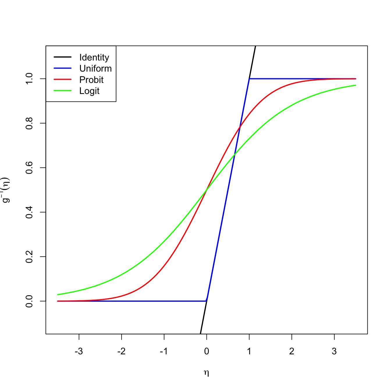
Figure 5.4: Transformations \(g^{-1}\) associated to different link functions. The transformations \(g^{-1}\) map the response of a linear regression \(\eta=\beta_0+\beta_1x_1+\cdots+\beta_px_p\) to \(\lbrack 0,1\rbrack.\)

The logistic transformation is the most employed due to its tractability, interpretability, and smoothness¹⁴⁶. Its inverse, \(g:[0,1]\longrightarrow\mathbb{R},\) is known as the logit function:

\[\begin{align*} \mathrm{logit}(p):=\mathrm{logistic}^{-1}(p)=\log\left(\frac{p}{1-p}\right). \end{align*}\]

In conclusion, with the logit link function we can map the domain of \(Y\) to \(\mathbb{R}\) in order to apply a linear model. The logistic model can be then equivalently stated as

\[\begin{align} \mathbb{E}[Y|X_1=x_1,\ldots,X_p=x_p]&=\mathrm{logistic}(\eta)=\frac{1}{1+e^{-\eta}}\tag{5.4}, \end{align}\]

or as

\[\begin{align} \mathrm{logit}(\mathbb{E}[Y|X_1=x_1,\ldots,X_p=x_p])=\eta \tag{5.5} \end{align}\]

where recall that

\[\begin{align*} \eta=\beta_0+\beta_1x_1+\cdots+\beta_px_p. \end{align*}\]

There is a clear interpretation of the role of the linear predictor \(\eta\) in (5.4) when we come back to (5.3):

• If \(\eta=0,\) then \(\mathbb{P}[Y=1|X_1=x_1,\ldots,X_p=x_p]=\frac{1}{2}\) (\(Y=1\) and \(Y=0\) are equally likely).
• If \(\eta<0,\) then \(\mathbb{P}[Y=1|X_1=x_1,\ldots,X_p=x_p]<\frac{1}{2}\) (\(Y=1\) is less likely).
• If \(\eta>0,\) then \(\mathbb{P}[Y=1|X_1=x_1,\ldots,X_p=x_p]>\frac{1}{2}\) (\(Y=1\) is more likely).

To be more precise on the interpretation of the coefficients we need to introduce the odds. The odds is an equivalent way of expressing the distribution of probabilities in a binary variable \(Y.\) Instead of using \(p\) to characterize the distribution of \(Y,\) we can use

\[\begin{align} \mathrm{odds}(Y):=\frac{p}{1-p}=\frac{\mathbb{P}[Y=1]}{\mathbb{P}[Y=0]}.\tag{5.6} \end{align}\]

The odds is thus the ratio between the probability of success and the probability of failure¹⁴⁷. It is extensively used in betting¹⁴⁸ due to its better interpretability¹⁴⁹. Conversely, if the odds of \(Y\) is given, we can easily know what is the probability of success \(p,\) using the inverse of (5.6)¹⁵⁰:

\[\begin{align*} p=\mathbb{P}[Y=1]=\frac{\text{odds}(Y)}{1+\text{odds}(Y)}. \end{align*}\]

Recall that the odds is a number in \([0,+\infty].\) The \(0\) and \(+\infty\) values are attained for \(p=0\) and \(p=1,\) respectively. The log-odds (or logit) is a number in \([-\infty,+\infty].\)

We can rewrite (5.4) in terms of the odds (5.6)¹⁵¹ so we get:

\[\begin{align} \mathrm{odds}(Y|X_1=x_1,\ldots,X_p=x_p)=e^{\eta}=e^{\beta_0}e^{\beta_1x_1}\cdots e^{\beta_px_p}.\tag{5.7} \end{align}\]

Alternatively, taking logarithms, we have the log-odds (or logit)

\[\begin{align} \log(\mathrm{odds}(Y|X_1=x_1,\ldots,X_p=x_p))=\beta_0+\beta_1x_1+\cdots+\beta_px_p.\tag{5.8} \end{align}\]

The conditional log-odds (5.8) plays the role of the conditional mean for multiple linear regression. Therefore, we have an analogous interpretation for the coefficients:

• \(\beta_0\): is the log-odds when \(X_1=\ldots=X_p=0.\)
• \(\beta_j,\) \(1\leq j\leq p\): is the additive increment of the log-odds for an increment of one unit in \(X_j=x_j,\) provided that the remaining variables \(X_1,\ldots,X_{j-1},X_{j+1},\ldots,X_p\) do not change.

The log-odds is not as easy to interpret as the odds. For that reason, an equivalent way of interpreting the coefficients, this time based on (5.7), is:

• \(e^{\beta_0}\): is the odds when \(X_1=\ldots=X_p=0.\)
• \(e^{\beta_j},\) \(1\leq j\leq p\): is the multiplicative increment of the odds for an increment of one unit in \(X_j=x_j,\) provided that the remaining variables \(X_1,\ldots,X_{j-1},X_{j+1},\ldots,X_p\) do not change. If the increment in \(X_j\) is of \(r\) units, then the multiplicative increment in the odds is \((e^{\beta_j})^r.\)

As a consequence of this last interpretation, we have:

If \(\beta_j>0\) (respectively, \(\beta_j<0\)) then \(e^{\beta_j}>1\) (\(e^{\beta_j}<1\)) in (5.7). Therefore, an increment of one unit in \(X_j,\) provided that the remaining variables do not change, results in a positive (negative) increment in the odds and in \(\mathbb{P}[Y=1|X_1=x_1,\ldots,X_p=x_p].\)

Case study application

In the Challenger case study we used fail.field as an indicator of whether “there was at least an incident with the O-rings” (1 = yes, 0 = no). Let’s see if the temperature was associated with O-ring incidents (Q1). For that, we compute the logistic regression of fail.field on temp and we plot the fitted logistic curve.

# Logistic regression: computed with glm and family = "binomial"
nasa <- glm(fail.field ~ temp, family = "binomial", data = challenger)

# Plot data
plot(challenger$temp, challenger$fail.field, xlim = c(-1, 30),
     xlab = "Temperature", ylab = "Incident probability")

# Draw the fitted logistic curve
x <- seq(-1, 30, l = 200)
y <- exp(-(nasa$coefficients[1] + nasa$coefficients[2] * x))
y <- 1 / (1 + y)
lines(x, y, col = 2, lwd = 2)

# The Challenger
points(-0.6, 1, pch = 16)
text(-0.6, 1, labels = "Challenger", pos = 4)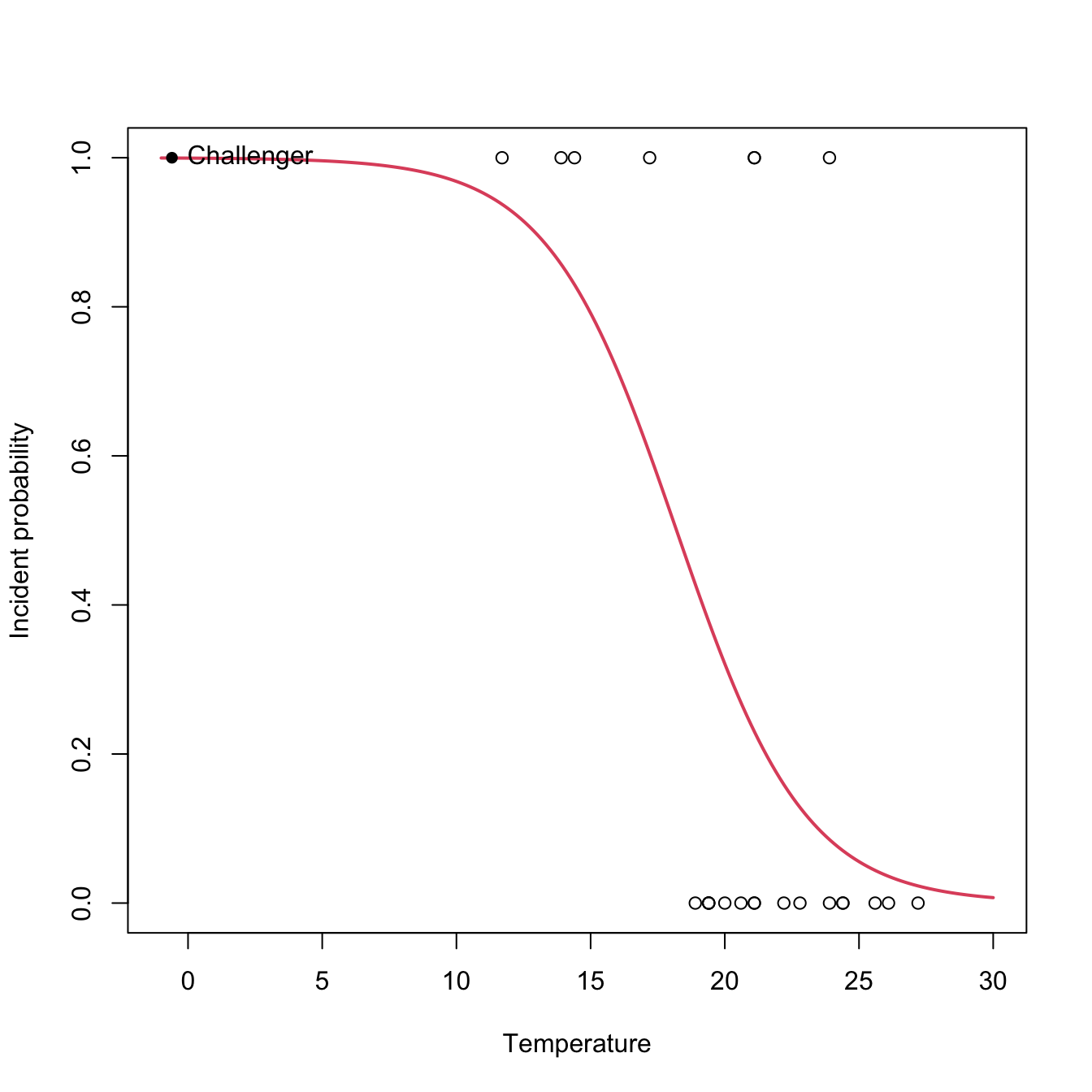

At the sight of this curve and the summary it seems that the temperature was affecting the probability of an O-ring incident (Q1). Let’s quantify this statement and answer Q2 by looking to the coefficients of the model:

# Exponentiated coefficients ("odds ratios")
exp(coef(nasa))
##  (Intercept)         temp 
## 1965.9743592    0.6592539

The exponentials of the estimated coefficients are:

• \(e^{\hat\beta_0}=1965.974.\) This means that, when the temperature is zero, the fitted odds is \(1965.974,\) so the (estimated) probability of having an incident (\(Y=1\)) is \(1965.974\) times larger than the probability of not having an incident (\(Y=0\)). Or, in other words, the probability of having an incident at temperature zero is \(\frac{1965.974}{1965.974+1}=0.999.\)
• \(e^{\hat\beta_1}=0.659.\) This means that each Celsius degree increment on the temperature multiplies the fitted odds by a factor of \(0.659\approx\frac{2}{3},\) hence reducing it.

However, for the moment we cannot say whether these findings are significant or are just an artifact of the randomness of the data, since we do not have information on the variability of the estimates of \(\boldsymbol{\beta}.\) We will need inference for that.

Estimation by maximum likelihood

The estimation of \(\boldsymbol{\beta}\) from a sample \(\{(\mathbf{x}_i,Y_i)\}_{i=1}^n\;\)¹⁵² is done by Maximum Likelihood Estimation (MLE). As it can be seen in Appendix A.2, in the linear model, under the assumptions mentioned in Section 2.3, MLE is equivalent to least squares estimation. In the logistic model, we assume that¹⁵³

\[\begin{align*} Y_i|(X_{1}=x_{i1},\ldots,X_{p}=x_{ip})\sim \mathrm{Ber}(\mathrm{logistic}(\eta_i)),\quad i=1,\ldots,n, \end{align*}\]

where \(\eta_i:=\beta_0+\beta_1x_{i1}+\cdots+\beta_px_{ip}.\) Denoting \(p_i(\boldsymbol{\beta}):=\mathrm{logistic}(\eta_i),\) the log-likelihood of \(\boldsymbol{\beta}\) is

\[\begin{align} \ell(\boldsymbol{\beta})&=\log\left(\prod_{i=1}^np_i(\boldsymbol{\beta})^{Y_i}(1-p_i(\boldsymbol{\beta}))^{1-Y_i}\right)\nonumber\\ &=\sum_{i=1}^n\left[Y_i\log(p_i(\boldsymbol{\beta}))+(1-Y_i)\log(1-p_i(\boldsymbol{\beta}))\right].\tag{5.9} \end{align}\]

The ML estimate of \(\boldsymbol{\beta}\) is

\[\begin{align*} \hat{\boldsymbol{\beta}}:=\arg\max_{\boldsymbol{\beta}\in\mathbb{R}^{p+1}}\ell(\boldsymbol{\beta}). \end{align*}\]

Unfortunately, due to the nonlinearity of (5.9), there is no explicit expression for \(\hat{\boldsymbol{\beta}}\) and it has to be obtained numerically by means of an iterative procedure. We will see that with more detail in the next section. Just be aware that this iterative procedure may fail to converge in low sample size situations with perfect classification, where the likelihood might be numerically unstable.

Figure 5.5: The logistic regression fit and its dependence on \(\beta_0\) (horizontal displacement) and \(\beta_1\) (steepness of the curve). Recall the effect of the sign of \(\beta_1\) in the curve: if positive, the logistic curve has an ‘s’ form; if negative, the form is a reflected ‘s’. Application available here.

Figure 5.5 shows how the log-likelihood changes with respect to the values for \((\beta_0,\beta_1)\) in three data patterns. The data of the illustration has been generated with the next chunk of code.

# Data
set.seed(34567)
x <- rnorm(50, sd = 1.5)
y1 <- -0.5 + 3 * x
y2 <- 0.5 - 2 * x
y3 <- -2 + 5 * x
y1 <- rbinom(50, size = 1, prob = 1 / (1 + exp(-y1)))
y2 <- rbinom(50, size = 1, prob = 1 / (1 + exp(-y2)))
y3 <- rbinom(50, size = 1, prob = 1 / (1 + exp(-y3)))

# Data
dataMle <- data.frame(x = x, y1 = y1, y2 = y2, y3 = y3)

For fitting a logistic model we employ glm, which has the syntax glm(formula = response ~ predictor, family = "binomial", data = data), where response is a binary variable. Note that family = "binomial" is referring to the fact that the response is a binomial variable (since it is a Bernoulli). Let’s check that indeed the coefficients given by glm are the ones that maximize the likelihood given in the animation of Figure 5.5. We do so for y1 ~ x.

# Call glm
mod <- glm(y1 ~ x, family = "binomial", data = dataMle)
mod$coefficients
## (Intercept)           x 
##  -0.1691947   2.4281626

# -loglik(beta)
minusLogLik <- function(beta) {
  p <- 1 / (1 + exp(-(beta[1] + beta[2] * x)))
  -sum(y1 * log(p) + (1 - y1) * log(1 - p))
}

# Optimization using as starting values beta = c(0, 0)
opt <- optim(par = c(0, 0), fn = minusLogLik)
opt
## $par
## [1] -0.1691366  2.4285119
## 
## $value
## [1] 14.79376
## 
## $counts
## function gradient 
##       73       NA 
## 
## $convergence
## [1] 0
## 
## $message
## NULL

# Visualization of the log-likelihood surface
beta0 <- seq(-3, 3, l = 50)
beta1 <- seq(-2, 8, l = 50)
L <- matrix(nrow = length(beta0), ncol = length(beta1))
for (i in seq_along(beta0)) {
  for (j in seq_along(beta1)) {
    L[i, j] <- minusLogLik(c(beta0[i], beta1[j]))
  }
}
filled.contour(beta0, beta1, -L, color.palette = viridis::viridis,
               xlab = expression(beta[0]), ylab = expression(beta[1]),
               plot.axes = {
                 axis(1); axis(2)
                 points(mod$coefficients[1], mod$coefficients[2],
                        col = 2, pch = 16)
                 points(opt$par[1], opt$par[2], col = 4)
               })

Figure 5.6: Log-likelihood surface \(\ell(\beta_0,\beta_1)\) and its global maximum \((\hat\beta_0,\hat\beta_1).\)

# The plot.axes argument is a hack to add graphical information within the
# coordinates of the main panel (behind filled.contour there is a layout()...)

For the regressions y2 ~ x and y3 ~ x, do the following:

1. Check that the true \(\boldsymbol{\beta}\) is close to maximizing the likelihood computed in Figure 5.5.
2. Plot the fitted logistic curve and compare it with the one in Figure 5.5.

The extension of the logistic model to the case of a categorical response with more than two levels is sketched in Appendix A.3.

5.2.2 General case

The same idea we used in logistic regression, namely transforming the conditional expectation of \(Y\) into something that can be modeled by a linear model (this is, a quantity that lives in \(\mathbb{R}\)), can be generalized. This raises the family of generalized linear models, which extends the linear model to different kinds of response variables and provides a convenient parametric framework.

The first ingredient is a link function \(g,\) that is monotonic and differentiable, which is going to produce a transformed expectation¹⁵⁴ to be modeled by a linear combination of the predictors:

\[\begin{align*} g\left(\mathbb{E}[Y|X_1=x_1,\ldots,X_p=x_p]\right)=\eta \end{align*}\]

or, equivalently,

\[\begin{align*} \mathbb{E}[Y|X_1=x_1,\ldots,X_p=x_p]&=g^{-1}(\eta), \end{align*}\]

where

\[\begin{align*} \eta:=\beta_0+\beta_1x_1+\cdots+\beta_px_p \end{align*}\]

is the linear predictor.

The second ingredient of generalized linear models is a distribution for \(Y|(X_1,\ldots,X_p),\) just as the linear model assumes normality or the logistic model assumes a Bernoulli random variable. Thus, we have two linked generalizations with respect to the usual linear model:

1. The conditional mean may be modeled by a transformation \(g^{-1}\) of the linear predictor \(\eta.\)
2. The distribution of \(Y|(X_1,\ldots,X_p)\) may be different from the normal.

Generalized linear models are intimately related with the exponential family^{155 156}, which is the family of distributions with pdf expressible as

\[\begin{align} f(y;\theta,\phi)=\exp\left\{\frac{y\theta-b(\theta)}{a(\phi)}+c(y,\phi)\right\},\tag{5.10} \end{align}\]

where \(a(\cdot),\) \(b(\cdot),\) and \(c(\cdot,\cdot)\) are specific functions. If \(Y\) has the pdf (5.10), then we write \(Y\sim\mathrm{E}(\theta,\phi,a,b,c).\) If the scale parameter \(\phi\) is known, this is an exponential family with canonical parameter \(\theta\) (if \(\phi\) is unknown, then it may or not may be a two-parameter exponential family).

Distributions from the exponential family have some nice properties. Importantly, if \(Y\sim\mathrm{E}(\theta,\phi,a,b,c),\) then

\[\begin{align} \mu:=\mathbb{E}[Y]=b'(\theta),\quad \sigma^2:=\mathbb{V}\mathrm{ar}[Y]=b''(\theta)a(\phi).\tag{5.11} \end{align}\]

The canonical link function is the function \(g\) that transforms \(\mu=b'(\theta)\) into the canonical parameter \(\theta\). For \(\mathrm{E}(\theta,\phi,a,b,c),\) this happens if

\[\begin{align} \theta=g(\mu) \tag{5.12} \end{align}\]

or, more explicitly due to (5.11), if

\[\begin{align} g(\mu)=(b')^{-1}(\mu). \tag{5.13} \end{align}\]

In the case of canonical link function, the one-line summary of the generalized linear model is (independence is implicit)

\[\begin{align} Y|(X_1=x_1,\ldots,X_p=x_p)\sim\mathrm{E}(\eta,\phi,a,b,c).\tag{5.14} \end{align}\]

Expression (5.14) gives insight on what a generalized linear model does:

1. Select a member of the exponential family in (5.10) for modeling \(Y.\)
2. The canonical link function \(g\) is \(g(\mu)=(b')^{-1}(\mu).\) In this case, \(\theta=g(\mu).\)
3. The generalized linear model associated to the member of the exponential family and \(g\) models the conditional \(\theta,\) given \(X_1,\ldots,X_n,\) by means of the linear predictor \(\eta.\) This is equivalent to modeling the conditional \(\mu\) by means of \(g^{-1}(\eta).\)

The linear model arises as a particular case of (5.14) with

\[\begin{align*} a(\phi)=\phi,\quad b(\theta)=\frac{\theta^2}{2},\quad c(y,\phi)=-\frac{1}{2}\left\{\frac{y^2}{\phi}+\log(2\pi\phi)\right\}, \end{align*}\]

and scale parameter \(\phi=\sigma^2.\) In this case, \(\mu=\theta\) and the canonical link function \(g\) is the identity.

Show that the normal, Bernoulli, exponential, and Poisson distributions are members of the exponential family. For that, express their pdfs in terms of (5.10) and identify who is \(\theta\) and \(\phi.\)

Show that the binomial and gamma (which includes exponential and chi-squared) distributions are members of the exponential family. For that, express their pdfs in terms of (5.10) and identify who is \(\theta\) and \(\phi.\)

The following table lists some useful generalized linear models. Recall that the linear and logistic models of Sections 2.2.3 and 5.2.1 are obtained from the first and second rows, respectively.

Support of \(Y\)	Generating distribution	Link \(g(\mu)\)	Expectation \(g^{-1}(\eta)\)	Scale \(\phi\)	Distribution of \(Y\vert\mathbf{X}=\mathbf{x}\)
\(\mathbb{R}\)	\(\mathcal{N}(\mu,\sigma^2)\)	\(\mu\)	\(\eta\)	\(\sigma^2\)	\(\mathcal{N}(\eta,\sigma^2)\)
\(\{0,1\}\)	\(\mathrm{Ber}(p)\)	\(\mathrm{logit}(\mu)\)	\(\mathrm{logistic}(\eta)\)	\(1\)	\(\mathrm{Ber}\left(\mathrm{logistic}(\eta)\right)\)
\(\{0,\ldots,N\}\)	\(\mathrm{B}(N,p)\)	\(\log\left(\frac{\mu}{N-\mu}\right)\)	\(N\cdot\mathrm{logistic}(\eta)\)	\(1\)	\(\mathrm{B}(N,\mathrm{logistic}(\eta))\)
\(\{0,1,\ldots\}\)	\(\mathrm{Pois}(\lambda)\)	\(\log(\mu)\)	\(e^\eta\)	\(1\)	\(\mathrm{Pois}(e^{\eta})\)
\((0,\infty)\)	\(\Gamma(a,\nu)\;\)157	\(-\frac{1}{\mu}\)	\(-\frac{1}{\eta}\)	\(\frac{1}{\nu}\)	\(\Gamma(-\eta \nu,\nu)\;\)158

Obtain the canonical link function for the exponential distribution \(\mathrm{Exp}(\lambda).\) What is the scale parameter? What is the distribution of \(Y\vert(X_1=x_1,\ldots,X_p=x_p)\) in such model?

Poisson regression

Poisson regression is usually employed for modeling count data that arises from the recording of the frequencies of a certain phenomenon. It considers that

\[\begin{align*} Y|(X_1=x_1,\ldots,X_p=x_p)\sim\mathrm{Pois}(e^{\eta}), \end{align*}\]

this is,

\[\begin{align} \mathbb{E}[Y|X_1=x_1,\ldots,X_p=x_p]&=\lambda(Y|X_1=x_1,\ldots,X_p=x_p)\nonumber\\ &=e^{\beta_0+\beta_1x_1+\cdots+\beta_px_p}.\tag{5.15} \end{align}\]

Let’s see how to apply a Poisson regression. For that aim we consider the species (download) dataset. The goal is to analyze whether the Biomass and the pH (a factor) of the terrain are influential on the number of Species. Incidentally, it will serve to illustrate that the use of factors within glm is completely analogous to what we did with lm.

# Read data
species <- read.table("species.txt", header = TRUE)
species$pH <- as.factor(species$pH)

# Plot data
plot(Species ~ Biomass, data = species, col = as.numeric(pH))
legend("topright", legend = c("High pH", "Medium pH", "Low pH"),
       col = c(1, 3, 2), lwd = 2) # colors according to as.numeric(pH)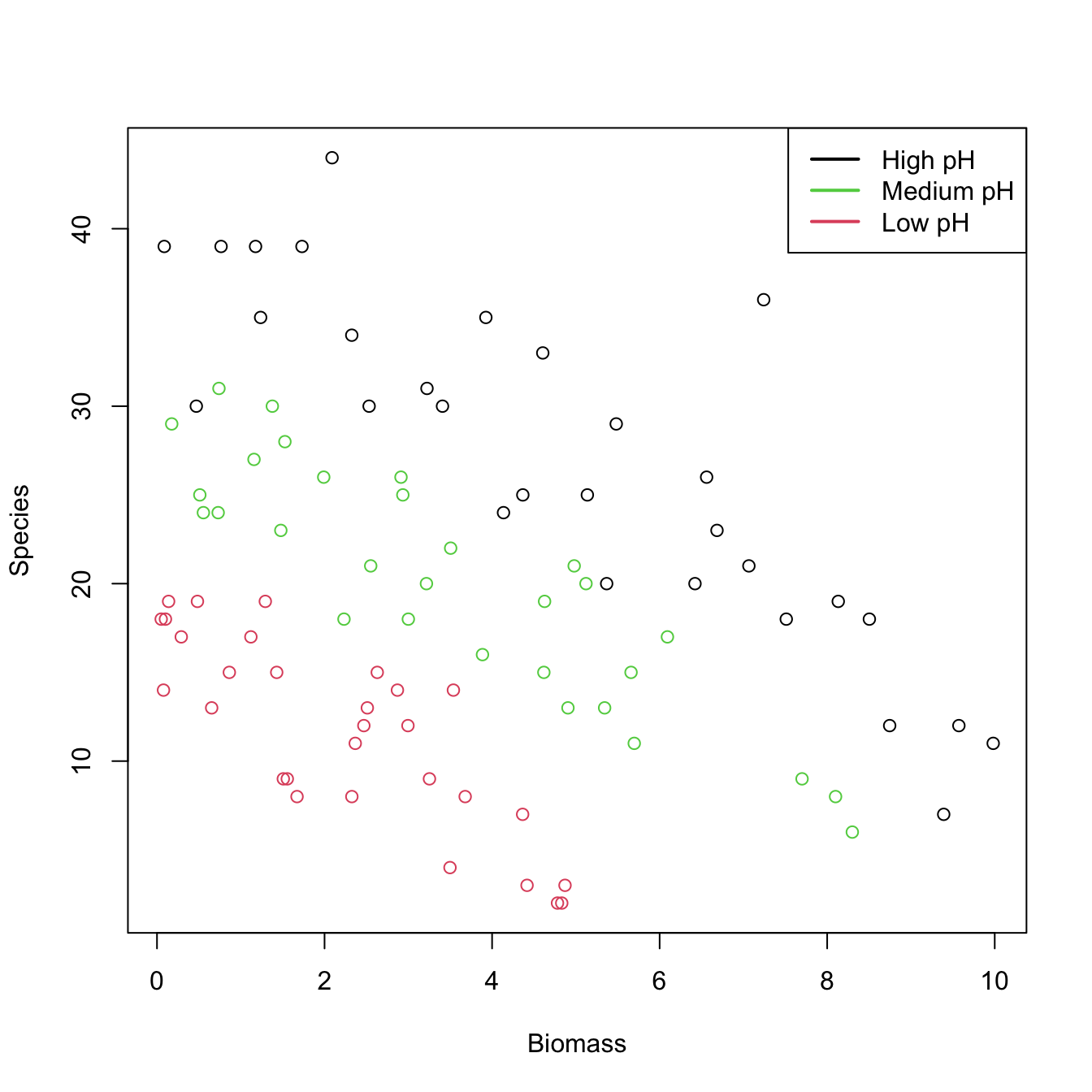

# Fit Poisson regression
species1 <- glm(Species ~ ., data = species, family = poisson)
summary(species1)
## 
## Call:
## glm(formula = Species ~ ., family = poisson, data = species)
## 
## Deviance Residuals: 
##     Min       1Q   Median       3Q      Max  
## -2.5959  -0.6989  -0.0737   0.6647   3.5604  
## 
## Coefficients:
##             Estimate Std. Error z value Pr(>|z|)    
## (Intercept)  3.84894    0.05281  72.885  < 2e-16 ***
## pHlow       -1.13639    0.06720 -16.910  < 2e-16 ***
## pHmed       -0.44516    0.05486  -8.114 4.88e-16 ***
## Biomass     -0.12756    0.01014 -12.579  < 2e-16 ***
## ---
## Signif. codes:  0 '***' 0.001 '**' 0.01 '*' 0.05 '.' 0.1 ' ' 1
## 
## (Dispersion parameter for poisson family taken to be 1)
## 
##     Null deviance: 452.346  on 89  degrees of freedom
## Residual deviance:  99.242  on 86  degrees of freedom
## AIC: 526.43
## 
## Number of Fisher Scoring iterations: 4
# Took 4 iterations of the IRLS

# Interpretation of the coefficients:
exp(species1$coefficients)
## (Intercept)       pHlow       pHmed     Biomass 
##  46.9433686   0.3209744   0.6407222   0.8802418
# - 46.9433 is the average number of species when Biomass = 0 and the pH is high
# - For each increment in one unit in Biomass, the number of species decreases
#   by a factor of 0.88 (12% reduction)
# - If pH decreases to med (low), then the number of species decreases by a factor
#   of 0.6407 (0.3209)

# With interactions
species2 <- glm(Species ~ Biomass * pH, data = species, family = poisson)
summary(species2)
## 
## Call:
## glm(formula = Species ~ Biomass * pH, family = poisson, data = species)
## 
## Deviance Residuals: 
##     Min       1Q   Median       3Q      Max  
## -2.4978  -0.7485  -0.0402   0.5575   3.2297  
## 
## Coefficients:
##               Estimate Std. Error z value Pr(>|z|)    
## (Intercept)    3.76812    0.06153  61.240  < 2e-16 ***
## Biomass       -0.10713    0.01249  -8.577  < 2e-16 ***
## pHlow         -0.81557    0.10284  -7.931 2.18e-15 ***
## pHmed         -0.33146    0.09217  -3.596 0.000323 ***
## Biomass:pHlow -0.15503    0.04003  -3.873 0.000108 ***
## Biomass:pHmed -0.03189    0.02308  -1.382 0.166954    
## ---
## Signif. codes:  0 '***' 0.001 '**' 0.01 '*' 0.05 '.' 0.1 ' ' 1
## 
## (Dispersion parameter for poisson family taken to be 1)
## 
##     Null deviance: 452.346  on 89  degrees of freedom
## Residual deviance:  83.201  on 84  degrees of freedom
## AIC: 514.39
## 
## Number of Fisher Scoring iterations: 4
exp(species2$coefficients)
##   (Intercept)       Biomass         pHlow         pHmed Biomass:pHlow Biomass:pHmed 
##    43.2987424     0.8984091     0.4423865     0.7178730     0.8563910     0.9686112
# - If pH decreases to med (low), then the effect of the biomass in the number
#   of species decreases by a factor of 0.9686 (0.8564). The higher the pH, the
#   stronger the effect of the Biomass in Species

# Draw fits
plot(Species ~ Biomass, data = species, col = as.numeric(pH))
legend("topright", legend = c("High pH", "Medium pH", "Low pH"),
       col = c(1, 3, 2), lwd = 2) # colors according to as.numeric(pH)

# Without interactions
bio <- seq(0, 10, l = 100)
z <- species1$coefficients[1] + species1$coefficients[4] * bio
lines(bio, exp(z), col = 1)
lines(bio, exp(species1$coefficients[2] + z), col = 2)
lines(bio, exp(species1$coefficients[3] + z), col = 3)

# With interactions seems to provide a significant improvement
bio <- seq(0, 10, l = 100)
z <- species2$coefficients[1] + species2$coefficients[2] * bio
lines(bio, exp(z), col = 1, lty = 2)
lines(bio, exp(species2$coefficients[3] + species2$coefficients[5] * bio + z),
      col = 2, lty = 2)
lines(bio, exp(species2$coefficients[4] + species2$coefficients[6] * bio + z),
      col = 3, lty = 2)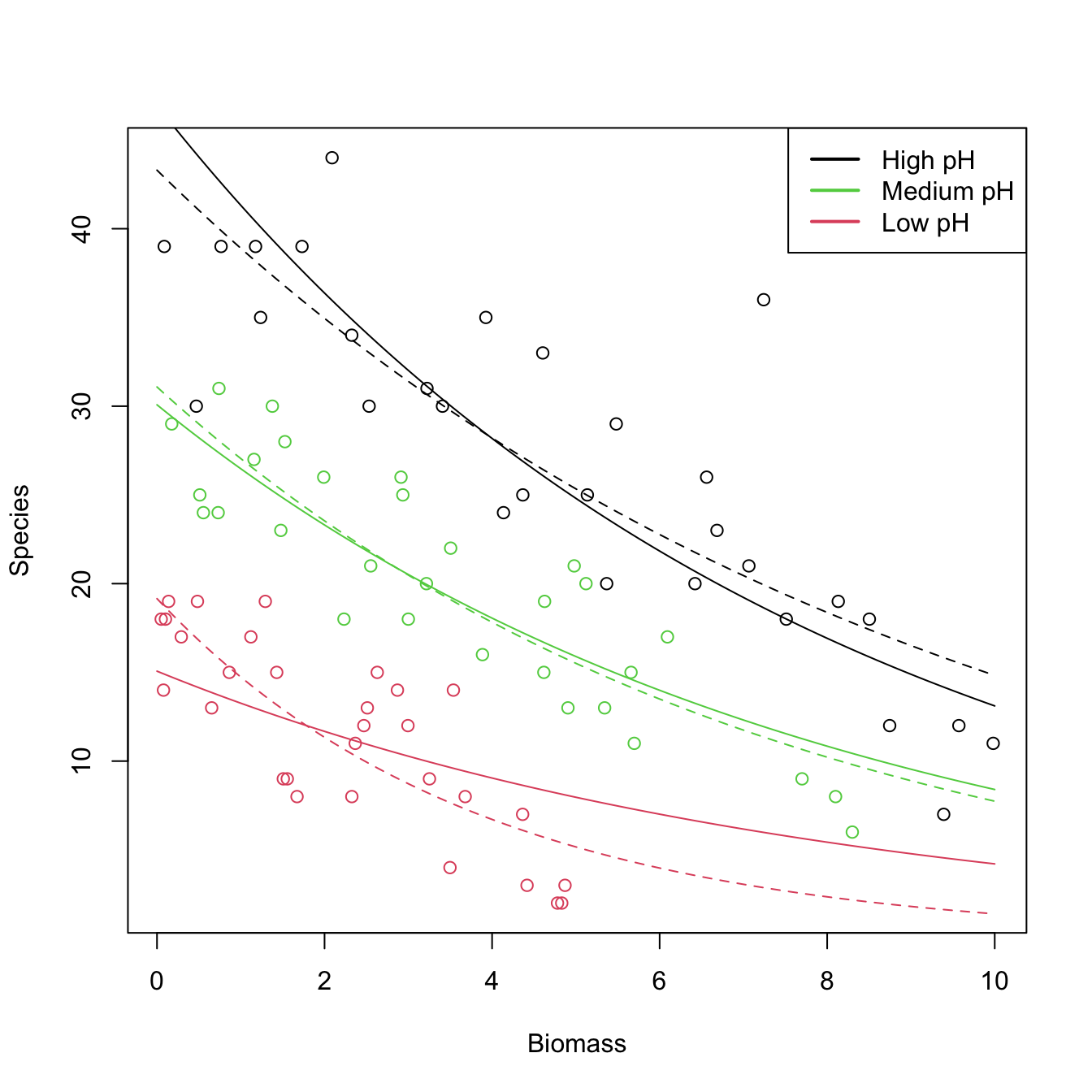

For the challenger dataset, do the following:

1. Do a Poisson regression of the total number of incidents, nfails.field + nfails.nozzle, on temp.
2. Plot the data and the fitted Poisson regression curve.
3. Predict the expected number of incidents at temperatures \(-0.6\) and \(11.67.\)

Binomial regression

Binomial regression is an extension of logistic regression that allows to model discrete responses \(Y\) in \(\{0,1,\ldots,N\},\) where \(N\) is fixed. In its most vanilla version, it considers the model

\[\begin{align} Y|(X_1=x_1,\ldots,X_p=x_p)\sim\mathrm{B}(N,\mathrm{logistic}(\eta)),\tag{5.16} \end{align}\]

this is,

\[\begin{align} \mathbb{E}[Y|X_1=x_1,\ldots,X_p=x_p]=N\cdot\mathrm{logistic}(\eta).\tag{5.17} \end{align}\]

Comparing (5.17) with (5.4), it is clear that the logistic regression is a particular case with \(N=1.\) The interpretation of the coefficients is therefore clear from the interpretation of (5.4), given that \(\mathrm{logistic}(\eta)\) models the probability of success of each of the \(N\) experiments of the binomial \(\mathrm{B}(N,\mathrm{logistic}(\eta)).\)

The extra flexibility that binomial regression has offers interesting applications. First, we can use (5.16) as an approach to model proportions¹⁵⁹ \(Y/N\in[0,1].\) In this case, (5.17) becomes¹⁶⁰

\[\begin{align*} \mathbb{E}[Y/N|X_1=x_1,\ldots,X_p=x_p]=\mathrm{logistic}(\eta). \end{align*}\]

Second, we can let \(N\) be dependent on the predictors to accommodate group structures, perhaps the most common usage of binomial regression:

\[\begin{align} Y|\mathbf{X}=\mathbf{x}\sim\mathrm{B}(N_\mathbf{x},\mathrm{logistic}(\eta)),\tag{5.18} \end{align}\]

where the size of the binomial distribution, \(N_\mathbf{x},\) depends on the values of the predictors. For example, imagine that the predictors are two quantitative variables and two dummy variables encoding three categories. Then \(\mathbf{X}=(X_1,X_2, D_1,D_2)'\) and \(\mathbf{x}=(x_1,x_2, d_1,d_2)'.\) In this case, \(N_\mathbf{x}\) could for example take the form

\[\begin{align*} N_\mathbf{x}=\begin{cases} 30,&d_1=0,d_2=0,\\ 25,&d_1=1,d_2=0,\\ 50,&d_1=0,d_2=1, \end{cases} \end{align*}\]

that is, we have a different number of experiments on each category, and we want to model the number (or, equivalently, the proportion) of successes for each one, also taking into account the effects of other qualitative variables. This is a very common situation in practice, when one encounters the sample version of (5.18):

\[\begin{align} Y_i|\mathbf{X}_i=\mathbf{x}_i\sim\mathrm{B}(N_i,\mathrm{logistic}(\eta_i)),\quad i=1,\ldots,n.\tag{5.19} \end{align}\]

Let’s see an example of binomial regression that illustrates the particular usage of glm() in this case. The example is a data application from Wood (2006) featuring different binomial sizes. It employs the heart (download) dataset. The goal is to investigate whether the level of creatinine kinase level present in the blood, ck, is a good diagnostic for determining if a patient is likely to have a future heart attack. The number of patients that did not have a heart attack (ok) and that had a heart attack (ha) was established after ck was measured. In total, there are \(226\) patients that have been aggregated into \(n=12\;\)¹⁶¹ categories of different sizes that have been created according to the average level of ck. Table 5.2 shows the data.

# Read data
heart <- read.table("heart.txt", header = TRUE)

# Sizes for each observation (Ni's)
heart$Ni <- heart$ok + heart$ha

# Proportions of patients with heart attacks
heart$prop <- heart$ha / (heart$ha + heart$ok)

Table 5.2: The heart dataset with \(N_i\) (Ni) and \(Y_i/N_i\) (prop) added.

ck	ha	ok	Ni	prop
20	2	88	90	0.022
60	13	26	39	0.333
100	30	8	38	0.789
140	30	5	35	0.857
180	21	0	21	1.000
220	19	1	20	0.950
260	18	1	19	0.947
300	13	1	14	0.929
340	19	1	20	0.950
380	15	0	15	1.000
420	7	0	7	1.000
460	8	0	8	1.000

# Plot of proportions versus ck: twelve observations, each requiring
# Ni patients to determine the proportion
plot(heart$ck, heart$prop, xlab = "Creatinine kinase level",
     ylab = "Proportion of heart attacks")

# Fit binomial regression: recall the cbind() to pass the number of successes
# and failures
heart1 <- glm(cbind(ha, ok) ~ ck, family = binomial, data = heart)
summary(heart1)
## 
## Call:
## glm(formula = cbind(ha, ok) ~ ck, family = binomial, data = heart)
## 
## Deviance Residuals: 
##      Min        1Q    Median        3Q       Max  
## -3.08184  -1.93008   0.01652   0.41772   2.60362  
## 
## Coefficients:
##              Estimate Std. Error z value Pr(>|z|)    
## (Intercept) -2.758358   0.336696  -8.192 2.56e-16 ***
## ck           0.031244   0.003619   8.633  < 2e-16 ***
## ---
## Signif. codes:  0 '***' 0.001 '**' 0.01 '*' 0.05 '.' 0.1 ' ' 1
## 
## (Dispersion parameter for binomial family taken to be 1)
## 
##     Null deviance: 271.712  on 11  degrees of freedom
## Residual deviance:  36.929  on 10  degrees of freedom
## AIC: 62.334
## 
## Number of Fisher Scoring iterations: 6

# Alternatively: put proportions as responses, but then it is required to
# inform about the binomial size of each observation
heart1 <- glm(prop ~ ck, family = binomial, data = heart, weights = Ni)
summary(heart1)
## 
## Call:
## glm(formula = prop ~ ck, family = binomial, data = heart, weights = Ni)
## 
## Deviance Residuals: 
##      Min        1Q    Median        3Q       Max  
## -3.08184  -1.93008   0.01652   0.41772   2.60362  
## 
## Coefficients:
##              Estimate Std. Error z value Pr(>|z|)    
## (Intercept) -2.758358   0.336696  -8.192 2.56e-16 ***
## ck           0.031244   0.003619   8.633  < 2e-16 ***
## ---
## Signif. codes:  0 '***' 0.001 '**' 0.01 '*' 0.05 '.' 0.1 ' ' 1
## 
## (Dispersion parameter for binomial family taken to be 1)
## 
##     Null deviance: 271.712  on 11  degrees of freedom
## Residual deviance:  36.929  on 10  degrees of freedom
## AIC: 62.334
## 
## Number of Fisher Scoring iterations: 6

# Add fitted line
ck <- 0:500
newdata <- data.frame(ck = ck)
logistic <- function(eta) 1 / (1 + exp(-eta))
lines(ck, logistic(cbind(1, ck) %*% heart1$coefficients))

# It seems that a polynomial fit could better capture the "wiggly" pattern
# of the data
heart2 <- glm(prop ~ poly(ck, 2, raw = TRUE), family = binomial, data = heart,
              weights = Ni)
heart3 <- glm(prop ~ poly(ck, 3, raw = TRUE), family = binomial, data = heart,
              weights = Ni)
heart4 <- glm(prop ~ poly(ck, 4, raw = TRUE), family = binomial, data = heart,
              weights = Ni)

# Best fit given by heart3
BIC(heart1, heart2, heart3, heart4)
##        df      BIC
## heart1  2 63.30371
## heart2  3 44.27018
## heart3  4 35.59736
## heart4  5 37.96360
summary(heart3)
## 
## Call:
## glm(formula = prop ~ poly(ck, 3, raw = TRUE), family = binomial, 
##     data = heart, weights = Ni)
## 
## Deviance Residuals: 
##      Min        1Q    Median        3Q       Max  
## -0.99572  -0.08966   0.07468   0.17815   1.61096  
## 
## Coefficients:
##                            Estimate Std. Error z value Pr(>|z|)    
## (Intercept)              -5.786e+00  9.268e-01  -6.243 4.30e-10 ***
## poly(ck, 3, raw = TRUE)1  1.102e-01  2.139e-02   5.153 2.57e-07 ***
## poly(ck, 3, raw = TRUE)2 -4.649e-04  1.381e-04  -3.367  0.00076 ***
## poly(ck, 3, raw = TRUE)3  6.448e-07  2.544e-07   2.535  0.01125 *  
## ---
## Signif. codes:  0 '***' 0.001 '**' 0.01 '*' 0.05 '.' 0.1 ' ' 1
## 
## (Dispersion parameter for binomial family taken to be 1)
## 
##     Null deviance: 271.7124  on 11  degrees of freedom
## Residual deviance:   4.2525  on  8  degrees of freedom
## AIC: 33.658
## 
## Number of Fisher Scoring iterations: 6

# All fits together
lines(ck, logistic(cbind(1, poly(ck, 2, raw = TRUE)) %*% heart2$coefficients),
      col = 2)
lines(ck, logistic(cbind(1, poly(ck, 3, raw = TRUE)) %*% heart3$coefficients),
      col = 3)
lines(ck, logistic(cbind(1, poly(ck, 4, raw = TRUE)) %*% heart4$coefficients),
      col = 4)
legend("bottomright", legend = c("Linear", "Quadratic", "Cubic", "Quartic"),
       col = 1:4, lwd = 2)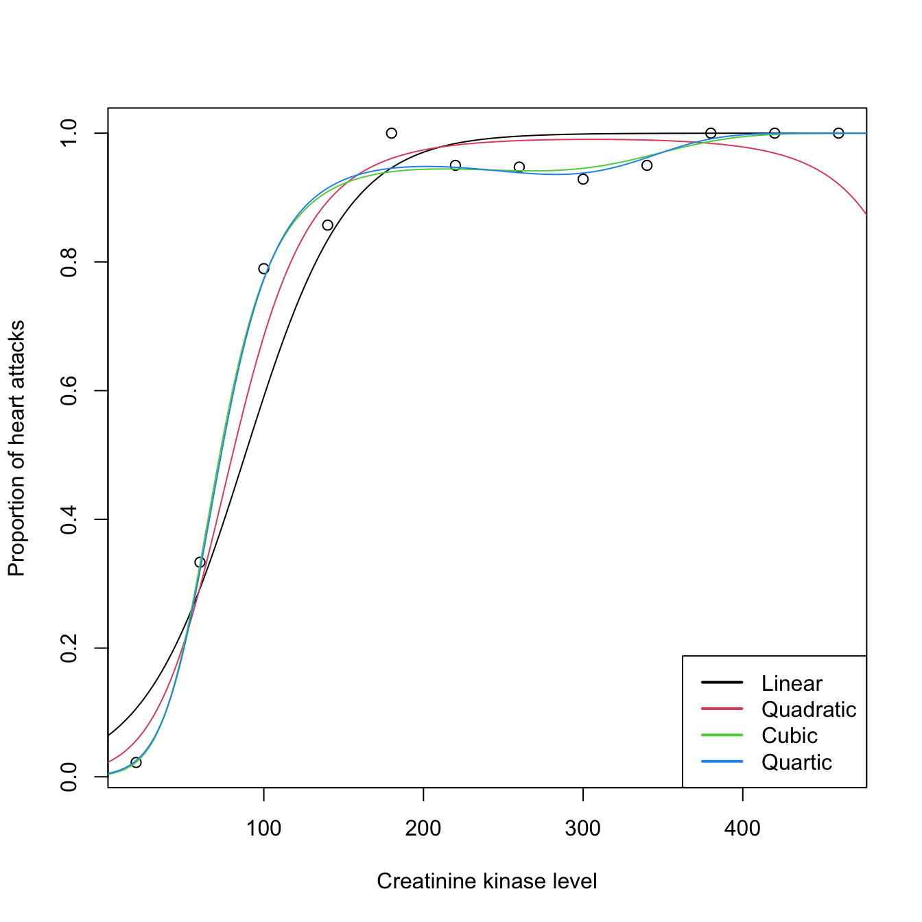

Estimation by maximum likelihood

The estimation of \(\boldsymbol{\beta}\) by MLE can be done in a unified framework, for all generalized linear models, thanks to the exponential family (5.10). Given \(\{(\mathbf{x}_i,Y_i)\}_{i=1}^n\)¹⁶², and employing a canonical link function (5.13), we have that

\[\begin{align*} Y_i|(X_1=x_{i1},\ldots,X_p=x_{ip})\sim\mathrm{E}(\theta_i,\phi,a,b,c),\quad i=1,\ldots,n, \end{align*}\]

where

\[\begin{align*} \theta_i&:=\eta_i:=\beta_0+\beta_1x_{i1}+\cdots+\beta_px_{ip},\\ \mu_i&:=\mathbb{E}[Y_i|X_1=x_{i1},\ldots,X_p=x_{ip}]=g^{-1}(\eta_i). \end{align*}\]

Then, the log-likelihood is

\[\begin{align} \ell(\boldsymbol{\beta})=\sum_{i=1}^n\left(\frac{Y_i\theta_i-b(\theta_i)}{a(\phi)}+c(Y_i,\phi)\right).\tag{5.20} \end{align}\]

Differentiating with respect to \(\boldsymbol{\beta}\) gives

\[\begin{align*} \frac{\partial \ell(\boldsymbol{\beta})}{\partial \boldsymbol{\beta}}=\sum_{i=1}^{n}\frac{\left(Y_i-b'(\theta_i)\right)}{a(\phi)}\frac{\partial \theta_i}{\partial \boldsymbol{\beta}} \end{align*}\]

which, exploiting the properties of the exponential family, can be reduced to

\[\begin{align} \frac{\partial \ell(\boldsymbol{\beta})}{\partial\boldsymbol{\beta}}=\sum_{i=1}^{n}\frac{(Y_i-\mu_i)}{g'(\mu_i)V_i}\mathbf{x}_i,\tag{5.21} \end{align}\]

where \(\mathbf{x}_i\) now represents the \(i\)-th row of the design matrix \(\mathbf{X}\) and \(V_i:=\mathbb{V}\mathrm{ar}[Y_i]=a(\phi)b''(\theta_i).\) Solving explicitly the system of equations \(\frac{\partial \ell(\boldsymbol{\beta})}{\partial\boldsymbol{\beta}}=\mathbf{0}\) is not possible in general and a numerical procedure is required. Newton–Raphson is usually employed, which is based in obtaining \(\boldsymbol{\beta}_\mathrm{new}\) from the linear system¹⁶³

\[\begin{align} \left.\frac{\partial^2 \ell(\boldsymbol{\beta})}{\partial \boldsymbol{\beta} \partial\boldsymbol{\beta}'}\right |_{\boldsymbol{\beta}=\boldsymbol{\beta}_\mathrm{old}}(\boldsymbol{\beta}_\mathrm{new} -\boldsymbol{\beta}_\mathrm{old})=-\left.\frac{\partial \ell(\boldsymbol{\beta})}{\partial \boldsymbol{\beta}} \right |_{\boldsymbol{\beta}=\boldsymbol{\beta}_\mathrm{old}}.\tag{5.22} \end{align}\]

A simplifying trick is to consider the expectation of \(\left.\frac{\partial^2 \ell(\boldsymbol{\beta})}{\partial \boldsymbol{\beta}\partial\boldsymbol{\beta}'}\right|_{\boldsymbol{\beta}=\boldsymbol{\beta}_\mathrm{old}}\) in (5.22), rather than its actual value. By doing so, we can arrive to a neat iterative algorithm called Iterative Reweighted Least Squares (IRLS). We use the following well-known property of the Fisher information matrix of the MLE theory:

\[\begin{align*} \mathbb{E}\left[\frac{\partial^2 \ell(\boldsymbol{\beta})}{\partial\boldsymbol{\beta} \partial\boldsymbol{\beta}'}\right]=-\mathbb{E}\left[\frac{\partial \ell(\boldsymbol{\beta})}{\partial \boldsymbol{\beta}}\left(\frac{\partial \ell(\boldsymbol{\beta})}{\partial \boldsymbol{\beta}}\right)'\right]. \end{align*}\]

Then, it can be seen that¹⁶⁴

\[\begin{align} \mathbb{E}\left[\left.\frac{\partial^2 \ell(\boldsymbol{\beta})}{\partial\boldsymbol{\beta}\partial\boldsymbol{\beta}'}\right|_{\boldsymbol{\beta}=\boldsymbol{\beta}_\mathrm{old}} \right]= -\sum_{i=1}^{n} w_i \mathbf{x}_i \mathbf{x}_i'=-\mathbf{X}' \mathbf{W} \mathbf{X},\tag{5.23} \end{align}\]

where \(w_i:=\frac{1}{V_i(g'(\mu_i))^2}\) and \(\mathbf{W}:=\mathrm{diag}(w_1,\ldots,w_n).\) Using this notation and from (5.21),

\[\begin{align} \left. \frac{\partial \ell(\boldsymbol{\beta})}{\partial \boldsymbol{\beta}} \right|_{\boldsymbol{\beta}=\boldsymbol{\beta}_\mathrm{old}}= \mathbf{X}'\mathbf{W}(\mathbf{Y}-\boldsymbol{\mu}_\mathrm{old})\mathbf{g}'(\boldsymbol{\mu}_\mathrm{old}),\tag{5.24} \end{align}\]

Substituting (5.23) and (5.24) in (5.22), we have:

\[\begin{align} \boldsymbol{\beta}_\mathrm{new}&=\boldsymbol{\beta}_\mathrm{old}-\mathbb{E}\left [\left.\frac{\partial^2 \ell(\boldsymbol{\beta})}{\partial\boldsymbol{\beta} \boldsymbol{\beta}'}\right|_{\boldsymbol{\beta}=\boldsymbol{\beta}_\mathrm{old}} \right]^{-1}\left. \frac{\partial \ell(\boldsymbol{\beta})}{\partial \boldsymbol{\beta}} \right|_{\boldsymbol{\beta}=\boldsymbol{\beta}_\mathrm{old}}\nonumber\\ &=\boldsymbol{\beta}_\mathrm{old}+(\mathbf{X}' \mathbf{W} \mathbf{X})^{-1}\mathbf{X}'\mathbf{W}(\mathbf{Y}-\boldsymbol{\mu}_\mathrm{old})\mathbf{g}'(\boldsymbol{\mu}_\mathrm{old})\nonumber\\ &=(\mathbf{X}' \mathbf{W} \mathbf{X})^{-1}\mathbf{X}'\mathbf{W} \mathbf{z},\tag{5.25} \end{align}\]

where \(\mathbf{z}:=\mathbf{X}\boldsymbol{\beta}_\mathrm{old}+(\mathbf{Y}-\boldsymbol{\mu}_\mathrm{old})\mathbf{g}'(\boldsymbol{\mu}_\mathrm{old})\) is the working vector.

As a consequence, fitting a generalized linear model by IRLS amounts to performing a series of weighted linear models with changing weights and responses given by the working vector. IRLS can be summarized as:

1. Set \(\boldsymbol{\beta}_\mathrm{old}\) with some initial estimation.
2. Compute \(\boldsymbol{\mu}_\mathrm{old},\) \(\mathbf{W},\) and \(\mathbf{z}.\)
3. Compute \(\boldsymbol{\beta}_\mathrm{new}\) using (5.25).
4. Set \(\boldsymbol{\beta}_\mathrm{old}\) as \(\boldsymbol{\beta}_\mathrm{new}.\)
5. Iterate Steps 2–4 until convergence, then set \(\hat{\boldsymbol{\beta}}=\boldsymbol{\beta}_\mathrm{new}.\)

In general, \(\mathbb{E}\left[\frac{\partial^2 \ell(\boldsymbol{\beta})}{\partial \boldsymbol{\beta} \partial\boldsymbol{\beta}'}\right]\neq \frac{\partial^2 \ell(\boldsymbol{\beta})}{\partial \boldsymbol{\beta} \partial\boldsymbol{\beta}'}.\) Therefore, IRLS in general departures from the standard Newton–Raphson. However, if the canonical link is used, it can be seen that the equality of \(\frac{\partial^2 \ell(\boldsymbol{\beta})}{\partial \boldsymbol{\beta} \partial\boldsymbol{\beta}'}\) with its expectation is guaranteed and IRLS is exactly the same as Newton–Raphson. In that case, \(w_i=\frac{1}{g'(\mu_i)}\) (which simplifies the computation of \(\mathbf{W}\) in the algorithm above).

References

Wood, S. N. 2006. Generalized Additive Models. Texts in Statistical Science Series. Boca Raton: Chapman & Hall/CRC. https://doi.org/10.1201/9781420010404.

---

143. Recall that a binomial variable with size \(n\) and probability \(p\), \(\mathrm{B}(n,p),\) is obtained by summing \(n\) independent \(\mathrm{Ber}(p),\) so \(\mathrm{Ber}(p)\) is the same distribution as \(\mathrm{B}(1,p).\)↩︎

144. Do not confuse this \(p\) with the number of predictors in the model, represented by \(p.\) The context should make unambiguous the use of \(p.\)↩︎

145. The fact that the logistic function is a cdf allows remembering that the logistic is to be applied to map \(\mathbb{R}\) into \([0,1],\) as opposed to the logit function.↩︎

146. And also, as we will see later, because it is the canonical link function.↩︎

147. Consequently, the name “odds” used in this context is singular, as it refers to a single ratio.↩︎

148. Recall that (traditionally) the result of a bet is binary: one either wins or loses it.↩︎

149. For example, if a horse \(Y\) has probability \(p=2/3\) of winning a race (\(Y=1\)), then the odds of the horse is \(\frac{p}{1-p}=\frac{2/3}{1/3}=2.\) This means that the horse has a probability of winning that is twice larger than the probability of losing. This is sometimes written as a \(2:1\) or \(2 \times 1\) (spelled “two-to-one”).↩︎

150. For the previous example: if the odds of the horse was \(5,\) then the probability of winning would be \(p=5/6.\)↩︎

151. To do so, apply (5.6) to (5.4) and use (5.3).↩︎

152. As in the linear model, we assume the randomness comes from the error present in \(Y\) once \(\mathbf{X}\) is given, not from the \(\mathbf{X},\) and we therefore denote \(\mathbf{x}_i\) to the \(i\)-th observation of \(\mathbf{X}.\)↩︎

153. Section 5.7 discusses in detail the assumptions of generalized linear models.↩︎

154. Notice that this approach is very different from directly transforming the response as \(g(Y),\) as outlined in Section 3.5.1. Indeed, in generalized linear models one transforms \(\mathbb{E}[Y|X_1,\ldots,X_p],\) not \(Y.\) Of course, \(g(\mathbb{E}[Y|X_1,\ldots,X_p])\neq \mathbb{E}[g(Y)|X_1,\ldots,X_p].\)↩︎

155. Not to be confused with the exponential distribution \(\mathrm{Exp}(\lambda),\) which is a member of the exponential family.↩︎

156. This is the so-called canonical form of the exponential family. Generalizations of the family are possible, though we do not consider them.↩︎

157. The pdf of a \(\Gamma(a,\nu)\) is \(f(x;a,p)=\frac{a^p}{\Gamma(\nu)}x^{\nu-1}e^{-ax},\) for \(a,\nu>0\) and \(x\in(0,\infty)\) (the pdf is zero otherwise). The expectation is \(\mathbb{E}\lbrack\Gamma(a,\nu)\rbrack=\frac{\nu}{a}.\)↩︎

158. If the argument \(-\eta \nu\) is not positive, then the probability assigned by \(\Gamma(-\eta \nu,\nu)\) is zero. This delicate case may complicate the estimation of the model. Valid starting values for \(\boldsymbol{\beta}\) are required.↩︎

159. Note this situation is very different from logistic regression, for which we either have observations with the values \(0\) or \(1.\) In binomial regression, we can naturally have proportions.↩︎

160. Clearly, \(\mathbb{E}[\mathrm{B}(N,p)/N]=p\) because \(\mathbb{E}[\mathrm{B}(N,p)]=Np.\)↩︎

161. The sample size here is \(n=12,\) not \(226.\) There are \(N_{1},\ldots,N_{12}\) binomial sizes corresponding to each observation, and \(\sum_{i=1}^{n}N_i=226.\)↩︎

162. We assume the randomness comes from the error present in \(Y\) once \(\mathbf{X}\) is given, not from the \(\mathbf{X}.\) This is implicit in the considered expectations.↩︎

163. The system stems from a first-order Taylor expansion of the function \(\frac{\partial \ell(\boldsymbol{\beta})}{\partial \boldsymbol{\beta}}:\mathbb{R}^{p+1}\rightarrow\mathbb{R}^{p+1}\) about the root \(\hat{\boldsymbol{\beta}},\) where \(\left.\frac{\partial \ell(\boldsymbol{\beta})}{\partial \boldsymbol{\beta}} \right |_{\boldsymbol{\beta}=\hat{\boldsymbol{\beta}}}=\mathbf{0}.\)↩︎

164. Recall that \(\mathbb{E}[(Y_i-\mu_i)(Y_j-\mu_j)]=\mathrm{Cov}[Y_i,Y_j]=\begin{cases}V_i,&i=j,\\0,&i\neq j,\end{cases}\) because of independence.↩︎