6.2 Kernel regression estimation

6.2.1 Nadaraya–Watson estimator

Our objective is to estimate the regression function $m:\mathbb{R}^p\rightarrow\mathbb{R}$ nonparametrically (recall that we are considering the simplest situation: one continuous predictor, so $p=1$). Due to its definition, we can rewrite $m$ as

$$\begin{align} m(x)=&\,\mathbb{E}[Y| X=x]\nonumber\\ =&\,\int y f_{Y| X=x}(y)\,\mathrm{d}y\nonumber\\ =&\,\frac{\int y f(x,y)\,\mathrm{d}y}{f_X(x)}.\tag{6.13} \end{align}$$

This expression shows an interesting point: the regression function can be computed from the joint density $f$ and the marginal $f_X.$ Therefore, given a sample $\{(X_i,Y_i)\}_{i=1}^n,$ a nonparametric estimate of $m$ may follow by replacing the previous densities by their kernel density estimators! From the previous section, we know how to do this using the multivariate and univariate kde’s given in (6.4) and (6.9), respectively. For the multivariate kde, we can consider the kde (6.12) based on product kernels for the two dimensional case and bandwidths $\mathbf{h}=(h_1,h_2)',$ which yields the estimate

$$\begin{align} \hat{f}(x,y;\mathbf{h})=\frac{1}{n}\sum_{i=1}^nK_{h_1}(x-X_{i})K_{h_2}(y-Y_{i})\tag{6.14} \end{align}$$

of the joint pdf of $(X,Y).$ On the other hand, considering the same bandwidth $h_1$ for the kde of $f_X,$ we have

$$\begin{align} \hat{f}_X(x;h_1)=\frac{1}{n}\sum_{i=1}^nK_{h_1}(x-X_{i}).\tag{6.15} \end{align}$$

We can therefore define the estimator of $m$ that results from replacing $f$ and $f_X$ in (6.13) by (6.14) and (6.15):

$$\begin{align*} \frac{\int y \hat{f}(x,y;\mathbf{h})\,\mathrm{d}y}{\hat{f}_X(x;h_1)}=&\,\frac{\int y \frac{1}{n}\sum_{i=1}^nK_{h_1}(x-X_i)K_{h_2}(y-Y_i)\,\mathrm{d}y}{\frac{1}{n}\sum_{i=1}^nK_{h_1}(x-X_i)}\\ =&\,\frac{\frac{1}{n}\sum_{i=1}^nK_{h_1}(x-X_i)\int y K_{h_2}(y-Y_i)\,\mathrm{d}y}{\frac{1}{n}\sum_{i=1}^nK_{h_1}(x-X_i)}\\ =&\,\frac{\frac{1}{n}\sum_{i=1}^nK_{h_1}(x-X_i)Y_i}{\frac{1}{n}\sum_{i=1}^nK_{h_1}(x-X_i)}\\ =&\,\sum_{i=1}^n\frac{K_{h_1}(x-X_i)}{\sum_{i=1}^nK_{h_1}(x-X_i)}Y_i. \end{align*}$$

The resulting estimator²⁰³ is the so-called Nadaraya–Watson²⁰⁴ estimator of the regression function:

$$\begin{align} \hat{m}(x;0,h):=\sum_{i=1}^n\frac{K_h(x-X_i)}{\sum_{i=1}^nK_h(x-X_i)}Y_i=\sum_{i=1}^nW^0_{i}(x)Y_i, \tag{6.16} \end{align}$$

where

$$\begin{align*} W^0_{i}(x):=\frac{K_h(x-X_i)}{\sum_{j=1}^nK_h(x-X_j)}. \end{align*}$$

The Nadaraya–Watson estimator can be seen as a weighted average of $Y_1,\ldots,Y_n$ by means of the set of weights $\{W_i(x)\}_{i=1}^n$ (they add to one). The set of varying weights depends on the evaluation point $x.$ That means that the Nadaraya–Watson estimator is a local mean of $Y_1,\ldots,Y_n$ about $X=x$ (see Figure 6.6).

Let’s implement from scratch the Nadaraya–Watson estimate to get a feeling of how it works in practice.

# A naive implementation of the Nadaraya-Watson estimator
mNW <- function(x, X, Y, h, K = dnorm) {

  # Arguments
  # x: evaluation points
  # X: vector (size n) with the predictors
  # Y: vector (size n) with the response variable
  # h: bandwidth
  # K: kernel

  # Matrix of size length(x) x n
  Kx <- sapply(X, function(Xi) K((x - Xi) / h) / h)

  # Weights
  W <- Kx / rowSums(Kx) # Column recycling!

  # Means at x ("drop" to drop the matrix attributes)
  drop(W %*% Y)

}

# Generate some data to test the implementation
set.seed(12345)
n <- 100
eps <- rnorm(n, sd = 2)
m <- function(x) x^2 * cos(x)
# m <- function(x) x - x^2 # Other possible regression function, works
# equally well
X <- rnorm(n, sd = 2)
Y <- m(X) + eps
xGrid <- seq(-10, 10, l = 500)

# Bandwidth
h <- 0.5

# Plot data
plot(X, Y)
rug(X, side = 1); rug(Y, side = 2)
lines(xGrid, m(xGrid), col = 1)
lines(xGrid, mNW(x = xGrid, X = X, Y = Y, h = h), col = 2)
legend("top", legend = c("True regression", "Nadaraya-Watson"),
       lwd = 2, col = 1:2)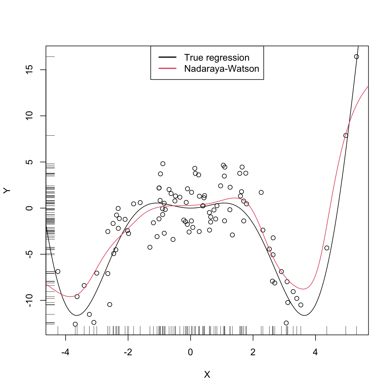

Figure 6.5: The Nadaraya–Watson estimator of an arbitrary regression function $m$.

Similarly to kernel density estimation, in the Nadaraya–Watson estimator the bandwidth has a prominent effect on the shape of the estimator, whereas the kernel is clearly less important. The code below illustrates the effect of varying $h$ using the manipulate::manipulate function.

# Simple plot of N-W for varying h's
manipulate::manipulate({

  # Plot data
  plot(X, Y)
  rug(X, side = 1); rug(Y, side = 2)
  lines(xGrid, m(xGrid), col = 1)
  lines(xGrid, mNW(x = xGrid, X = X, Y = Y, h = h), col = 2)
  legend("topright", legend = c("True regression", "Nadaraya-Watson"),
         lwd = 2, col = 1:2)

}, h = manipulate::slider(min = 0.01, max = 2, initial = 0.5, step = 0.01))

Implement your own version of the Nadaraya–Watson estimator in R and compare it with mNW. Focus only on the normal kernel and reduce the accuracy of the final computation up to 1e-7 to achieve better efficiency. Are you able to improve the speed of mNW? Use the microbenchmark::microbenchmark function to measure the running times for a sample with $n=10000.$

6.2.2 Local polynomial regression

The Nadaraya–Watson estimator can be seen as a particular case of a wider class of nonparametric estimators, the so called local polynomial estimators. Specifically, Nadaraya–Watson corresponds to performing a local constant fit. Let’s see this wider class of nonparametric estimators and their advantages with respect to the Nadaraya–Watson estimator.

The motivation for the local polynomial fit comes from attempting to find an estimator $\hat{m}$ of $m$ that “minimizes”²⁰⁵ the RSS

$$\begin{align} \sum_{i=1}^n(Y_i-\hat{m}(X_i))^2\tag{6.17} \end{align}$$

without assuming any particular form for the true $m.$ This is not achievable directly, since no knowledge on $m$ is available. Recall that what we did in parametric models was to assume a parametrization for $m.$ For example, in simple linear regression we assumed $m_{\boldsymbol{\beta}}(\mathbf{x})=\beta_0+\beta_1x,$ which allowed to tackle the minimization of (6.17) by means of solving

$$\begin{align*} m_{\hat{\boldsymbol{\beta}}}(\mathbf{x}):=\arg\min_{\boldsymbol{\beta}}\sum_{i=1}^n(Y_i-m_{\boldsymbol{\beta}}(X_i))^2. \end{align*}$$

The resulting $m_{\hat{\boldsymbol{\beta}}}$ is precisely the estimator that minimizes the RSS among all the linear estimators, that is, among the class of estimators that we have parametrized.

When $m$ has no available parametrization and can adopt any mathematical form, an alternative approach is required. The first step is to induce a local parametrization for $m.$ By a $p$-th²⁰⁶ order Taylor expression it is possible to obtain that, for $x$ close to $X_i,$

$$\begin{align} m(X_i)\approx&\, m(x)+m'(x)(X_i-x)+\frac{m''(x)}{2}(X_i-x)^2\nonumber\\ &+\cdots+\frac{m^{(p)}(x)}{p!}(X_i-x)^p.\tag{6.18} \end{align}$$

Then, replacing (6.18) in the population version of (6.17) that replaces $\hat{m}$ with $m,$ we have that

$$\begin{align} \sum_{i=1}^n\left(Y_i-\sum_{j=0}^p\frac{m^{(j)}(x)}{j!}(X_i-x)^j\right)^2.\tag{6.19} \end{align}$$

Expression (6.19) is still not workable: it depends on $m^{(j)}(x),$ $j=0,\ldots,p,$ which of course are unknown, as $m$ is unknown. The great idea is to set $\beta_j:=\frac{m^{(j)}(x)}{j!}$ and turn (6.19) into a linear regression problem where the unknown parameters are precisely $\boldsymbol{\beta}=(\beta_0,\beta_1,\ldots,\beta_p)'.$ Simply rewriting (6.19) using this idea gives

$$\begin{align} \sum_{i=1}^n\left(Y_i-\sum_{j=0}^p\beta_j(X_i-x)^j\right)^2.\tag{6.20} \end{align}$$

Now, estimates of $\boldsymbol{\beta}$ automatically produce estimates for $m^{(j)}(x)$! In addition, we know how to obtain an estimate $\hat{\boldsymbol{\beta}}$ that minimizes (6.20), since this is precisely the least squares problem studied in Section 2.2.3. The final touch is to weight the contributions of each datum $(X_i,Y_i)$ to the estimation of $m(x)$ according to the proximity of $X_i$ to $x.$²⁰⁷ We can achieve this precisely by kernels:

$$\begin{align} \hat{\boldsymbol{\beta}}_h:=\arg\min_{\boldsymbol{\beta}\in\mathbb{R}^{p+1}}\sum_{i=1}^n\left(Y_i-\sum_{j=0}^p\beta_j(X_i-x)^j\right)^2K_h(x-X_i).\tag{6.21} \end{align}$$

Solving (6.21) is easy once the proper notation is introduced. To that end, denote

$$\begin{align*} \mathbf{X}:=\begin{pmatrix} 1 & X_1-x & \cdots & (X_1-x)^p\\ \vdots & \vdots & \ddots & \vdots\\ 1 & X_n-x & \cdots & (X_n-x)^p\\ \end{pmatrix}_{n\times(p+1)} \end{align*}$$

and

$$\begin{align*} \mathbf{W}:=\mathrm{diag}(K_h(X_1-x),\ldots, K_h(X_n-x)),\quad \mathbf{Y}:=\begin{pmatrix} Y_1\\ \vdots\\ Y_n \end{pmatrix}_{n\times 1}. \end{align*}$$

Then we can re-express (6.21) into a weighted least squares problem²⁰⁸ whose exact solution is

$$\begin{align} \hat{\boldsymbol{\beta}}_h&=\arg\min_{\boldsymbol{\beta}\in\mathbb{R}^{p+1}} (\mathbf{Y}-\mathbf{X}\boldsymbol{\beta})'\mathbf{W}(\mathbf{Y}-\mathbf{X}\boldsymbol{\beta})\nonumber\\ &=(\mathbf{X}'\mathbf{W}\mathbf{X})^{-1}\mathbf{X}'\mathbf{W}\mathbf{Y}.\tag{6.22} \end{align}$$

The estimate²⁰⁹ for $m(x)$ is therefore computed as

$$\begin{align} \hat{m}(x;p,h):=&\,\hat{\beta}_{h,0}\nonumber\\ =&\,\mathbf{e}_1'(\mathbf{X}'\mathbf{W}\mathbf{X})^{-1}\mathbf{X}'\mathbf{W}\mathbf{Y}\nonumber\\ =&\,\sum_{i=1}^nW^p_{i}(x)Y_i\tag{6.23} \end{align}$$

where

$$\begin{align*} W^p_{i}(x):=\mathbf{e}_1'(\mathbf{X}'\mathbf{W}\mathbf{X})^{-1}\mathbf{X}'\mathbf{W}\mathbf{e}_i \end{align*}$$

and $\mathbf{e}_i$ is the $i$-th canonical vector. Just as the Nadaraya–Watson was, the local polynomial estimator is a weighted linear combination of the responses.

Two cases deserve special attention on (6.23):

• $p=0$ is the local constant estimator or the Nadaraya–Watson estimator. In this situation, the estimator has explicit weights, as we saw before:

  $$\begin{align*} W_i^0(x)=\frac{K_h(x-X_i)}{\sum_{j=1}^nK_h(x-X_j)}. \end{align*}$$

• $p=1$ is the local linear estimator, which has weights equal to:

  $$\begin{align*} W_i^1(x)=\frac{1}{n}\frac{\hat{s}_2(x;h)-\hat{s}_1(x;h)(X_i-x)}{\hat{s}_2(x;h)\hat{s}_0(x;h)-\hat{s}_1(x;h)^2}K_h(x-X_i), \end{align*}$$

  where $\hat{s}_r(x;h):=\frac{1}{n}\sum_{i=1}^n(X_i-x)^rK_h(x-X_i).$

Recall that the local polynomial fit is computationally more expensive than the local constant fit: $\hat{m}(x;p,h)$ is obtained as the solution of a weighted linear problem, whereas $\hat{m}(x;0,h)$ can be directly computed as a weighted mean of the responses.

Figure 6.6 illustrates the construction of the local polynomial estimator (up to cubic degree) and shows how $\hat\beta_0=\hat{m}(x;p,h),$ the intercept of the local fit, estimates $m$ at $x.$

Figure 6.6: Construction of the local polynomial estimator. The animation shows how local polynomial fits in a neighborhood of $x$ are combined to provide an estimate of the regression function, which depends on the polynomial degree, bandwidth, and kernel (gray density at the bottom). The data points are shaded according to their weights for the local fit at $x.$ Application available here.

The local polynomial estimator $\hat{m}(\cdot;p,h)$ of $m$ performs a series of weighted polynomial fits; as many as points $x$ on which $\hat{m}(\cdot;p,h)$ is to be evaluated.

An inefficient implementation of the local polynomial estimator can be done relatively straightforwardly from the previous insight and from expression (6.22). However, several R packages provide implementations, such as KernSmooth::locpoly and R’s loess²¹⁰ (but this one has a different control of the bandwidth plus a set of other modifications). Below are some examples of their usage.

# Generate some data
set.seed(123456)
n <- 100
eps <- rnorm(n, sd = 2)
m <- function(x) x^3 * sin(x)
X <- rnorm(n, sd = 1.5)
Y <- m(X) + eps
xGrid <- seq(-10, 10, l = 500)

# KernSmooth::locpoly fits
h <- 0.25
lp0 <- KernSmooth::locpoly(x = X, y = Y, bandwidth = h, degree = 0,
                           range.x = c(-10, 10), gridsize = 500)
lp1 <- KernSmooth::locpoly(x = X, y = Y, bandwidth = h, degree = 1,
                           range.x = c(-10, 10), gridsize = 500)
# Provide the evaluation points by range.x and gridsize

# loess fits
span <- 0.25 # The default span is 0.75, which works very bad in this scenario
lo0 <- loess(Y ~ X, degree = 0, span = span)
lo1 <- loess(Y ~ X, degree = 1, span = span)
# loess employs an "span" argument that plays the role of an variable bandwidth
# "span" gives the proportion of points of the sample that are taken into
# account for performing the local fit about x and then uses a triweight kernel
# (not a normal kernel) for weighting the contributions. Therefore, the final
# estimate differs from the definition of local polynomial estimator, although
# the principles in which are based are the same

# Prediction at x = 2
x <- 2
lp1$y[which.min(abs(lp1$x - x))] # Prediction by KernSmooth::locpoly
## [1] 5.445975
predict(lo1, newdata = data.frame(X = x)) # Prediction by loess
##        1 
## 5.379652
m(x) # Reality
## [1] 7.274379

# Plot data
plot(X, Y)
rug(X, side = 1); rug(Y, side = 2)
lines(xGrid, m(xGrid), col = 1)
lines(lp0$x, lp0$y, col = 2)
lines(lp1$x, lp1$y, col = 3)
lines(xGrid, predict(lo0, newdata = data.frame(X = xGrid)), col = 2, lty = 2)
lines(xGrid, predict(lo1, newdata = data.frame(X = xGrid)), col = 3, lty = 2)
legend("bottom", legend = c("True regression", "Local constant (locpoly)",
                            "Local linear (locpoly)", "Local constant (loess)",
                            "Local linear (loess)"),
       lwd = 2, col = c(1:3, 2:3), lty = c(rep(1, 3), rep(2, 2)))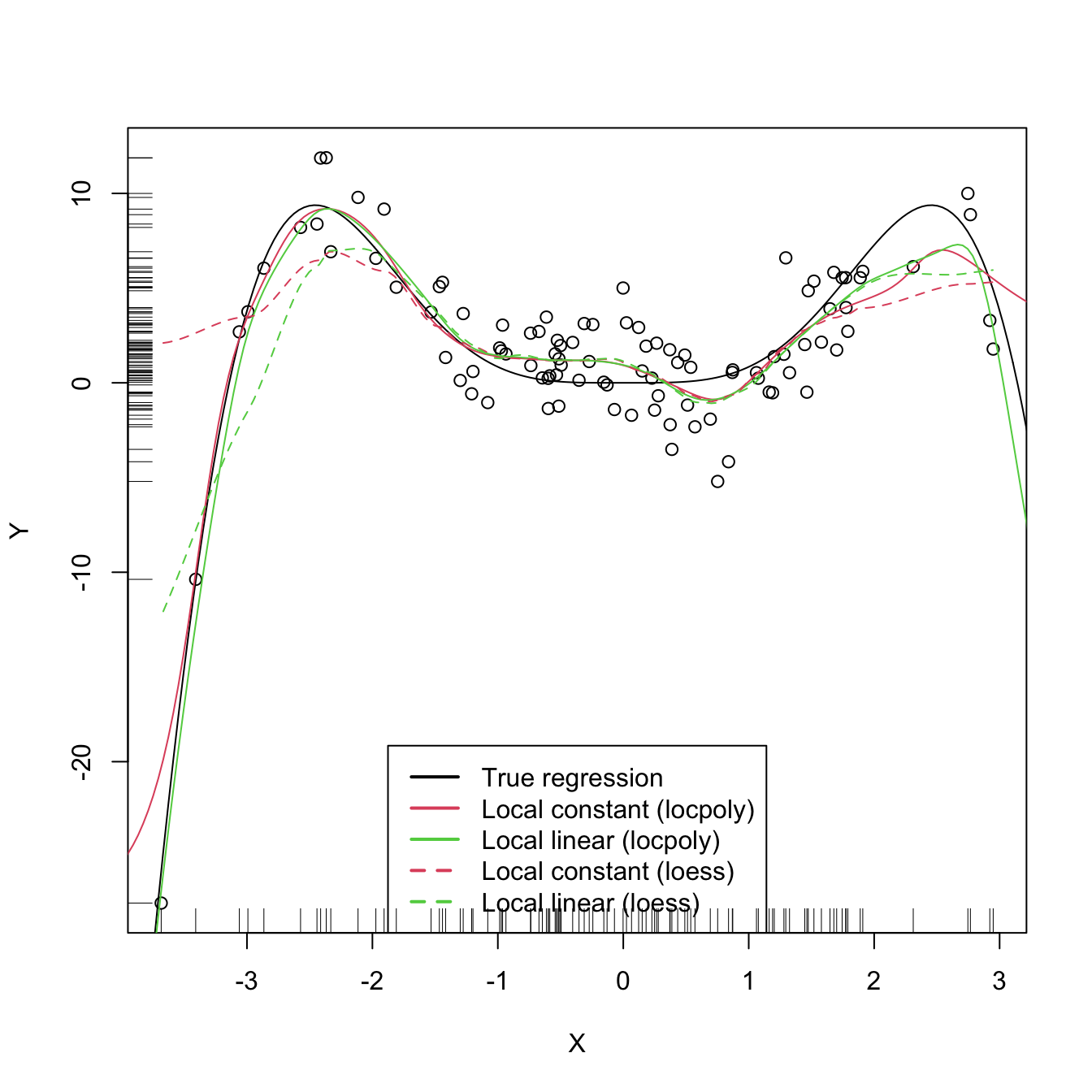

As with the Nadaraya–Watson, the local polynomial estimator heavily depends on $h.$

# Simple plot of local polynomials for varying h's
manipulate::manipulate({

  # Plot data
  lpp <- KernSmooth::locpoly(x = X, y = Y, bandwidth = h, degree = p,
                             range.x = c(-10, 10), gridsize = 500)
  plot(X, Y)
  rug(X, side = 1); rug(Y, side = 2)
  lines(xGrid, m(xGrid), col = 1)
  lines(lpp$x, lpp$y, col = p + 2)
  legend("bottom", legend = c("True regression", "Local polynomial fit"),
         lwd = 2, col = c(1, p + 2))

}, p = manipulate::slider(min = 0, max = 4, initial = 0, step = 1),
h = manipulate::slider(min = 0.01, max = 2, initial = 0.5, step = 0.01))

A more sophisticated framework for performing nonparametric estimation of the regression function is the np package, which we detail in Section 6.2.4. This package will be the chosen approach for the more challenging situation in which several predictors are present, since the former implementations do not escalate well for more than one predictor.

6.2.3 Asymptotic properties

What affects the performance of the local polynomial estimator? Is local linear estimation better than local constant estimation? What is the effect of $h$?

The purpose of this section is to provide some highlights on the questions above by examining the theoretical properties of the local polynomial estimator. This is achieved by examining the asymptotic bias and variance of the local linear and local constant estimators.²¹¹ For this goal, we consider the location-scale model for $Y$ and its predictor $X$:

$$\begin{align*} Y=m(X)+\sigma(X)\varepsilon, \end{align*}$$

where $\sigma^2(x):=\mathbb{V}\mathrm{ar}[Y| X=x]$ is the conditional variance of $Y$ given $X$ and $\varepsilon$ is such that $\mathbb{E}[\varepsilon| X=x]]=0$ and $\mathbb{V}\mathrm{ar}[\varepsilon| X=x]]=1.$ Note that since the conditional variance is not forced to be constant we are implicitly allowing for heteroscedasticity.

The following assumptions²¹² are the only requirements to perform the asymptotic analysis of the estimator:

• A1.²¹³ $m$ is twice continuously differentiable.
• A2.²¹⁴ $\sigma^2$ is continuous and positive.
• A3.²¹⁵ $f,$ the marginal pdf of $X,$ is continuously differentiable and bounded away from zero.²¹⁶
• A4.²¹⁷ The kernel $K$ is a symmetric and bounded pdf with finite second moment and is square integrable.
• A5.²¹⁸ $h=h_n$ is a deterministic sequence of bandwidths such that, when $n\to\infty,$ $h\to0$ and $nh\to\infty.$

The bias and variance are studied in their conditional versions on the predictor’s sample $X_1,\ldots,X_n.$ The reason for analyzing the conditional instead of the unconditional versions is avoiding technical difficulties that integration with respect to the predictor’s density may pose. This is in the spirit of what it was done in the parametric inference of Sections 2.4 and 5.3. The main result is the following, which provides useful insights on the effect of $p,$ $m,$ $f$ (standing from now on for the marginal pdf of $X$), and $\sigma^2$ in the performance of $\hat{m}(\cdot;p,h).$

Theorem 6.1 Under A1–A5, the conditional bias and variance of the local constant ($p=0$) and local linear ($p=1$) estimators are²¹⁹

$$\begin{align} \mathrm{Bias}[\hat{m}(x;p,h)| X_1,\ldots,X_n]&=B_p(x)h^2+o_\mathbb{P}(h^2),\tag{6.24}\\ \mathbb{V}\mathrm{ar}[\hat{m}(x;p,h)| X_1,\ldots,X_n]&=\frac{R(K)}{nhf(x)}\sigma^2(x)+o_\mathbb{P}((nh)^{-1}),\tag{6.25} \end{align}$$

where

$$\begin{align*} B_p(x):=\begin{cases} \frac{\mu_2(K)}{2}\left\{m''(x)+2\frac{m'(x)f'(x)}{f(x)}\right\},&\text{ if }p=0,\\ \frac{\mu_2(K)}{2}m''(x),&\text{ if }p=1. \end{cases} \end{align*}$$

The bias and variance expressions (6.24) and (6.25) yield very interesting insights:

1. Bias.

   • The bias decreases with $h$ quadratically for both $p=0,1.$ That means that small bandwidths $h$ give estimators with low bias, whereas large bandwidths provide largely biased estimators.

   • The bias at $x$ is directly proportional to $m''(x)$ if $p=1$ or affected by $m''(x)$ if $p=0.$ Therefore:

     • The bias is negative in regions where $m$ is concave, i.e., $\{x\in\mathbb{R}:m''(x)<0\}.$ These regions correspond to peaks and modes of $m$.
     • Conversely, the bias is positive in regions where $m$ is convex, i.e., $\{x\in\mathbb{R}:m''(x)>0\}.$ These regions correspond to valleys of $m$.
     • All in all, the “wilder” the curvature $m''$, the larger the bias and the harder to estimate $m$.

   • The bias for $p=0$ at $x$ is affected by $m'(x),$ $f'(x),$ and $f(x).$ All of them are quantities that are not present in the bias when $p=1.$ Precisely, for the local constant estimator, the lower the density $f(x),$ the larger the bias. Also, the faster $m$ and $f$ change at $x$ (derivatives), the larger the bias. Thus the bias of the local constant estimator is much more sensible to $m(x)$ and $f(x)$ than the local linear (which is only sensible to $m''(x)$). Particularly, the fact that the bias depends on $f'(x)$ and $f(x)$ is referred to as the design bias since it depends merely on the predictor’s distribution.

2. Variance.

   • The main term of the variance is the same for $p=0,1$. In addition, it depends directly on $\frac{\sigma^2(x)}{f(x)}.$ As a consequence, the lower the density, the more variable $\hat{m}(x;p,h)$ is.²²⁰ Also, the larger the conditional variance at $x,$ $\sigma^2(x),$ the more variable $\hat{m}(x;p,h)$ is.²²¹
   • The variance decreases at a factor of $(nh)^{-1}$. This is related with the so-called effective sample size $nh,$ which can be thought of as the amount of data in the neighborhood of $x$ that is employed for performing the regression.²²²

The main takeaway of the analysis of $p=0$ vs. $p=1$ is that $p=1$ has smaller bias than $p=0$ (but of the same order) while keeping the same variance as $p=0$.

An extended version of Theorem 6.1, given in Theorem 3.1 of Fan and Gijbels (1996), shows that this phenomenon extends to higher orders: odd order ($p=2\nu+1,$ $\nu\in\mathbb{N}$) polynomial fits introduce an extra coefficient for the polynomial fit that allows them to reduce the bias, while maintaining the same variance of the precedent even order ($p=2\nu$). So, for example, local cubic fits are preferred to local quadratic fits. This motivates the claim that local polynomial fitting is an “odd world” (Fan and Gijbels (1996)).

6.2.4 Bandwidth selection

Bandwidth selection, as for density estimation, has a crucial practical importance for kernel regression estimation. Several bandwidth selectors have been by following cross-validatory and plug-in ideas similar to the ones seen in Section 6.1.3. For simplicity, we briefly mention²²³ the DPI analogue for local linear regression for a single continuous predictor and focus mainly on least squares cross-validation, as it is a bandwidth selector that readily generalizes to the more complex settings of Section 6.3.

Following the derivation of the DPI for the kde, the first step is to define a suitable error criterion for the estimator $\hat{m}(\cdot;p,h).$ The conditional (on the sample of the predictor) MISE of $\hat{m}(\cdot;p,h)$ is often considered:

$$\begin{align*} \mathrm{MISE}[\hat{m}(\cdot;p,h)|X_1,\ldots,X_n]:=&\,\mathbb{E}\left[\int(\hat{m}(x;p,h)-m(x))^2f(x)\,\mathrm{d}x|X_1,\ldots,X_n\right]\\ =&\,\int\mathbb{E}\left[(\hat{m}(x;p,h)-m(x))^2|X_1,\ldots,X_n\right]f(x)\,\mathrm{d}x\\ =&\,\int\mathrm{MSE}\left[\hat{m}(x;p,h)|X_1,\ldots,X_n\right]f(x)\,\mathrm{d}x. \end{align*}$$

Observe that this definition is very similar to the kde’s MISE, except for the fact that $f$ appears weighting the quadratic difference: what matters is to minimize the estimation error of $m$ on the regions were the density of $X$ is higher. Recall also that the MISE follows by integrating the conditional MSE, which amounts to the squared bias (6.24) plus the variance (6.25) given in Theorem 6.1. These operations produce the conditional AMISE:

$$\begin{align*} \mathrm{AMISE}[\hat{m}(\cdot;p,h)|X_1,\ldots,X_n]=&\,h^2\int B_p(x)^2f(x)\,\mathrm{d}x+\frac{R(K)}{nh}\int\sigma^2(x)\,\mathrm{d}x \end{align*}$$

and, if $p=1,$ the resulting optimal AMISE bandwidth is

$$\begin{align*} h_\mathrm{AMISE}=\left[\frac{R(K)\int\sigma^2(x)\,\mathrm{d}x}{2\mu_2^2(K)\theta_{22}n}\right]^{1/5}, \end{align*}$$

where $\theta_{22}:=\int(m''(x))^2f(x)\,\mathrm{d}x.$

As happened in the density setting, the AMISE-optimal bandwidth cannot be readily employed, as knowledge about the “curvature” of $m,$ $\theta_{22},$ and about $\int\sigma^2(x)\,\mathrm{d}x$ is required. As with the DPI selector, a series of nonparametric estimations of $\theta_{22}$ and high-order curvature terms follow, concluding with a necessary estimation of a higher-order curvature based on a “block polynomial fit”.²²⁴ The estimation of $\int\sigma^2(x)\,\mathrm{d}x$ is carried out by assuming homoscedasticity and a compactly supported density $f.$ The resulting bandwidth selector, $\hat{h}_\mathrm{DPI},$ has a much faster convergence rate to $h_{\mathrm{MISE}}$ than cross-validatory selectors. However, it is notably more convoluted, and as a consequence is less straightforward to extend to more complex settings.

The DPI selector for the local linear estimator is implemented in KernSmooth::dpill.

# Generate some data
set.seed(123456)
n <- 100
eps <- rnorm(n, sd = 2)
m <- function(x) x^3 * sin(x)
X <- rnorm(n, sd = 1.5)
Y <- m(X) + eps
xGrid <- seq(-10, 10, l = 500)

# DPI selector
hDPI <- KernSmooth::dpill(x = X, y = Y)

# Fits
lp1 <- KernSmooth::locpoly(x = X, y = Y, bandwidth = 0.25, degree = 0,
                           range.x = c(-10, 10), gridsize = 500)
lp1DPI <- KernSmooth::locpoly(x = X, y = Y, bandwidth = hDPI, degree = 1,
                              range.x = c(-10, 10), gridsize = 500)

# Compare fits
plot(X, Y)
rug(X, side = 1); rug(Y, side = 2)
lines(xGrid, m(xGrid), col = 1)
lines(lp1$x, lp1$y, col = 2)
lines(lp1DPI$x, lp1DPI$y, col = 3)
legend("bottom", legend = c("True regression", "Local linear",
                            "Local linear (DPI)"),
       lwd = 2, col = 1:3)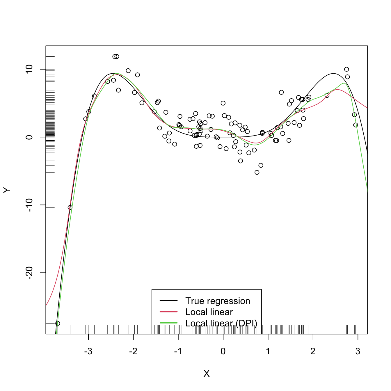

We turn now our attention to cross validation. Following an analogy with the fit of the linear model, we could look for the bandwidth $h$ such that it minimizes an RSS of the form

$$\begin{align} \frac{1}{n}\sum_{i=1}^n(Y_i-\hat{m}(X_i;p,h))^2.\tag{6.26} \end{align}$$

As it looks, this is a bad idea. Attempting to minimize (6.26) always leads to $h\approx 0$ that results in a useless interpolation of the data, as illustrated below.

# Grid for representing (6.26)
hGrid <- seq(0.1, 1, l = 200)^2
error <- sapply(hGrid, function(h) {
  mean((Y - mNW(x = X, X = X, Y = Y, h = h))^2)
})

# Error curve
plot(hGrid, error, type = "l")
rug(hGrid)
abline(v = hGrid[which.min(error)], col = 2)

As we know, the root of the problem is the comparison of $Y_i$ with $\hat{m}(X_i;p,h),$ since there is nothing forbidding $h\to0$ and as a consequence $\hat{m}(X_i;p,h)\to Y_i.$ As discussed in (3.17),²²⁵ a solution is to compare $Y_i$ with $\hat{m}_{-i}(X_i;p,h),$ the leave-one-out estimate of $m$ computed without the $i$-th datum $(X_i,Y_i),$ yielding the least squares cross-validation error

$$\begin{align} \mathrm{CV}(h)&:=\frac{1}{n}\sum_{i=1}^n(Y_i-\hat{m}_{-i}(X_i;p,h))^2\tag{6.27} \end{align}$$

and then choose

$$\begin{align*} \hat{h}_\mathrm{CV}&:=\arg\min_{h>0}\mathrm{CV}(h). \end{align*}$$

The optimization of (6.27) might seem as very computationally demanding, since it is required to compute $n$ regressions for just a single evaluation of the cross-validation function. There is, however, a simple and neat theoretical result that vastly reduces the computational complexity, at the price of increasing the memory demand. This trick allows to compute, with a single fit, the cross-validation function.

Proposition 6.1 For any $p\geq0,$ the weights of the leave-one-out estimator $\hat{m}_{-i}(x;p,h)=\sum_{\substack{j=1\\j\neq i}}^nW_{-i,j}^p(x)Y_j$ can be obtained from $\hat{m}(x;p,h)=\sum_{i=1}^nW_{i}^p(x)Y_i$:

$$\begin{align*} W_{-i,j}^p(x)=\frac{W^p_j(x)}{\sum_{\substack{k=1\\k\neq i}}^nW_k^p(x)}=\frac{W^p_j(x)}{1-W_i^p(x)}. \end{align*}$$

This implies that

$$\begin{align} \mathrm{CV}(h)=\frac{1}{n}\sum_{i=1}^n\left(\frac{Y_i-\hat{m}(X_i;p,h)}{1-W_i^p(X_i)}\right)^2.\tag{6.28} \end{align}$$

The result can be proved using that the weights $\{W_{i}^p(x)\}_{i=1}^n$ add to one, for any $x,$ and that $\hat{m}(x;p,h)$ is a linear combination²²⁶ of the responses $\{Y_i\}_{i=1}^n.$

Computing (6.28) requires evaluating the local polynomial estimator at the sample $\{X_i\}_{i=1}^n$ and obtaining $\{W_i^p(X_i)\}_{i=1}^n$ (which are needed for evaluating $\hat{m}(X_i;p,h)$). Both tasks can be achieved simultaneously from the $n\times n$ matrix $\left(W_{i}^p(X_j)\right)_{ij}$ and, if $p=0,$ directly from the symmetric $n\times n$ matrix $\left(K_h(X_i-X_j)\right)_{ij},$ whose storage costs $\mathcal{O}\left(\frac{n^2-n}{2}\right)$ (the diagonal is constant).

Let’s implement $\hat{h}_\mathrm{CV}$ for the Nadaraya–Watson estimator.

# Generate some data to test the implementation
set.seed(12345)
n <- 100
eps <- rnorm(n, sd = 2)
m <- function(x) x^2 + sin(x)
X <- rnorm(n, sd = 1.5)
Y <- m(X) + eps
xGrid <- seq(-10, 10, l = 500)

# Objective function
cvNW <- function(X, Y, h, K = dnorm) {

  sum(((Y - mNW(x = X, X = X, Y = Y, h = h, K = K)) /
         (1 - K(0) / colSums(K(outer(X, X, "-") / h))))^2)
  # Beware: outer() is not very memory-friendly!

}

# Find optimum CV bandwidth, with sensible grid
bw.cv.grid <- function(X, Y,
                       h.grid = diff(range(X)) * (seq(0.1, 1, l = 200))^2,
                       K = dnorm, plot.cv = FALSE) {

    obj <- sapply(h.grid, function(h) cvNW(X = X, Y = Y, h = h, K = K))
  h <- h.grid[which.min(obj)]
  if (plot.cv) {
    plot(h.grid, obj, type = "o")
    rug(h.grid)
    abline(v = h, col = 2, lwd = 2)
  }
  h

}

# Bandwidth
hCV <- bw.cv.grid(X = X, Y = Y, plot.cv = TRUE)

hCV
## [1] 0.3117806

# Plot result
plot(X, Y)
rug(X, side = 1); rug(Y, side = 2)
lines(xGrid, m(xGrid), col = 1)
lines(xGrid, mNW(x = xGrid, X = X, Y = Y, h = hCV), col = 2)
legend("top", legend = c("True regression", "Nadaraya-Watson"),
       lwd = 2, col = 1:2)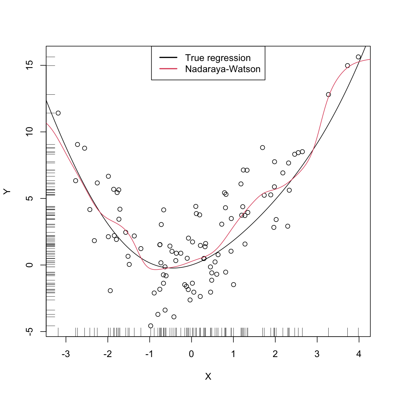

A more sophisticated cross-validation bandwidth selection can be achieved by np::npregbw and np::npreg, as shown in the code below.

# Turn off the "multistart" messages in the np package
options(np.messages = FALSE)

# np::npregbw computes by default the least squares CV bandwidth associated to
# a local constant fit
bw0 <- np::npregbw(formula = Y ~ X)

# Multiple initial points can be employed for minimizing the CV function (for
# one predictor, defaults to 1)
bw0 <- np::npregbw(formula = Y ~ X, nmulti = 2)

# The "rbandwidth" object contains many useful information, see ?np::npregbw for
# all the returned objects
bw0
## 
## Regression Data (100 observations, 1 variable(s)):
## 
##                       X
## Bandwidth(s): 0.3112962
## 
## Regression Type: Local-Constant
## Bandwidth Selection Method: Least Squares Cross-Validation
## Formula: Y ~ X
## Bandwidth Type: Fixed
## Objective Function Value: 5.368999 (achieved on multistart 1)
## 
## Continuous Kernel Type: Second-Order Gaussian
## No. Continuous Explanatory Vars.: 1
# Recall that the fit is very similar to hCV

# Once the bandwidth is estimated, np::npreg can be directly called with the
# "rbandwidth" object (it encodes the regression to be made, the data, the kind
# of estimator considered, etc). The hard work goes on np::npregbw, not on
# np::npreg
kre0 <- np::npreg(bw0)
kre0
## 
## Regression Data: 100 training points, in 1 variable(s)
##                       X
## Bandwidth(s): 0.3112962
## 
## Kernel Regression Estimator: Local-Constant
## Bandwidth Type: Fixed
## 
## Continuous Kernel Type: Second-Order Gaussian
## No. Continuous Explanatory Vars.: 1

# The evaluation points of the estimator are by default the predictor's sample
# (which is not sorted!)
# The evaluation of the estimator is given in "mean"
plot(kre0$eval$X, kre0$mean)

# The evaluation points can be changed using "exdat"
kre0 <- np::npreg(bw0, exdat = xGrid)

# Plot directly the fit via plot() -- it employs different evaluation points
# than exdat
plot(kre0, col = 2, type = "o")
points(X, Y)
rug(X, side = 1); rug(Y, side = 2)
lines(xGrid, m(xGrid), col = 1)
lines(kre0$eval$xGrid, kre0$mean, col = 3, type = "o", pch = 16, cex = 0.5)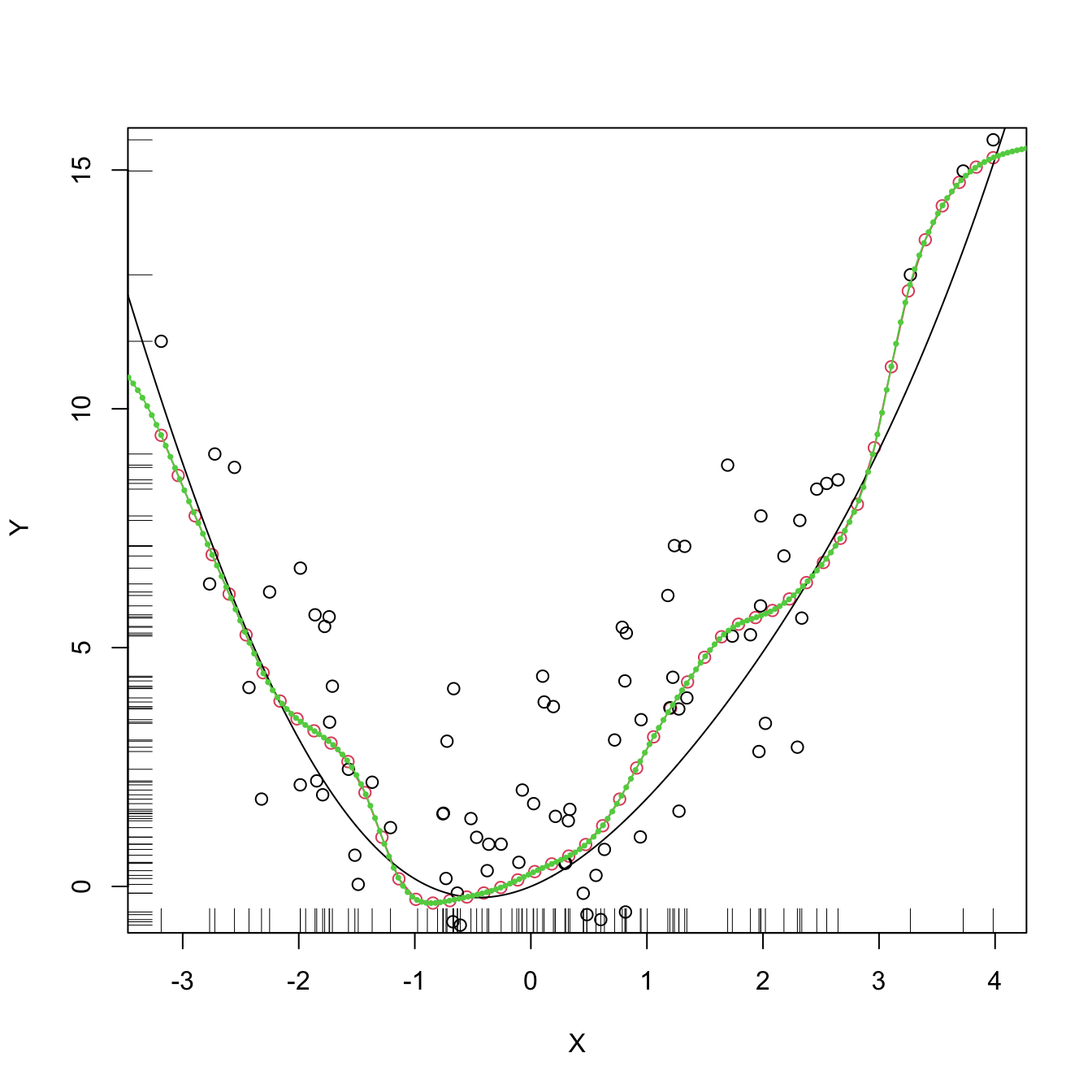

# Using the evaluation points

# Local linear fit -- find first the CV bandwidth
bw1 <- np::npregbw(formula = Y ~ X, regtype = "ll")
# regtype = "ll" stands for "local linear", "lc" for "local constant"

# Local linear fit
kre1 <- np::npreg(bw1, exdat = xGrid)

# Comparison
plot(X, Y)
rug(X, side = 1); rug(Y, side = 2)
lines(xGrid, m(xGrid), col = 1)
lines(kre0$eval$xGrid, kre0$mean, col = 2)
lines(kre1$eval$xGrid, kre1$mean, col = 3)
legend("top", legend = c("True regression", "Nadaraya-Watson", "Local linear"),
       lwd = 2, col = 1:3)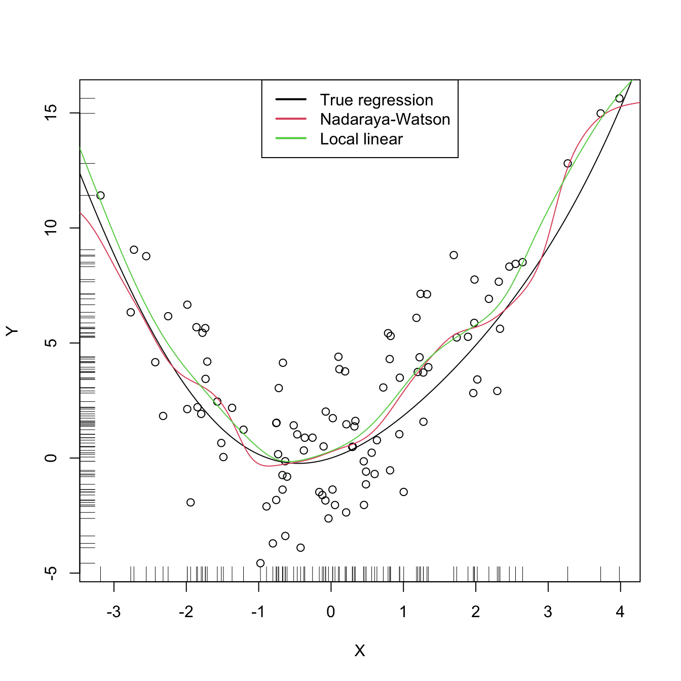

The adequate bandwidths for the local linear estimator are usually larger than the adequate bandwidths for the local constant estimator. The reason: the extra flexibility of the local linear estimator allows to adapt faster to variations in $m,$ whereas the local constant estimator can only achieve this by shrinking the neighborhood about $x$ by means of a small $h.$

There are more sophisticated options for bandwidth selection in np::npregbw. For example, the argument bwtype allows to estimate data-driven variable bandwidths $\hat{h}(x)$ that depend on the evaluation point $x,$ rather than fixed bandwidths $\hat{h},$ as we have considered. Roughly speaking, these variable bandwidths are related to the variable bandwidth $\hat{h}_k(x)$ that is necessary to contain the $k$ nearest neighbors $X_1,\ldots,X_k$ of $x$ in the neighborhood $(x-\hat{h}_k(x),x+\hat{h}_k(x)).$ There is a potential gain in employing variable bandwidths, as the estimator can adapt the amount of smoothing according to the density of the predictor. We do not investigate this approach in detail but just point to its implementation.

# Generate some data with bimodal density
set.seed(12345)
n <- 100
eps <- rnorm(2 * n, sd = 2)
m <- function(x) x^2 * sin(x)
X <- c(rnorm(n, mean = -2, sd = 0.5), rnorm(n, mean = 2, sd = 0.5))
Y <- m(X) + eps
xGrid <- seq(-10, 10, l = 500)

# Constant bandwidth
bwc <- np::npregbw(formula = Y ~ X, bwtype = "fixed", regtype = "ll")
krec <- np::npreg(bwc, exdat = xGrid)

# Variable bandwidths
bwg <- np::npregbw(formula = Y ~ X, bwtype = "generalized_nn", regtype = "ll")
kreg <- np::npreg(bwg, exdat = xGrid)
bwa <- np::npregbw(formula = Y ~ X, bwtype = "adaptive_nn", regtype = "ll")
krea <- np::npreg(bwa, exdat = xGrid)

# Comparison
plot(X, Y)
rug(X, side = 1); rug(Y, side = 2)
lines(xGrid, m(xGrid), col = 1)
lines(krec$eval$xGrid, krec$mean, col = 2)
lines(kreg$eval$xGrid, kreg$mean, col = 3)
lines(krea$eval$xGrid, krea$mean, col = 4)
legend("top", legend = c("True regression", "Fixed", "Generalized NN",
                         "Adaptive NN"),
       lwd = 2, col = 1:4)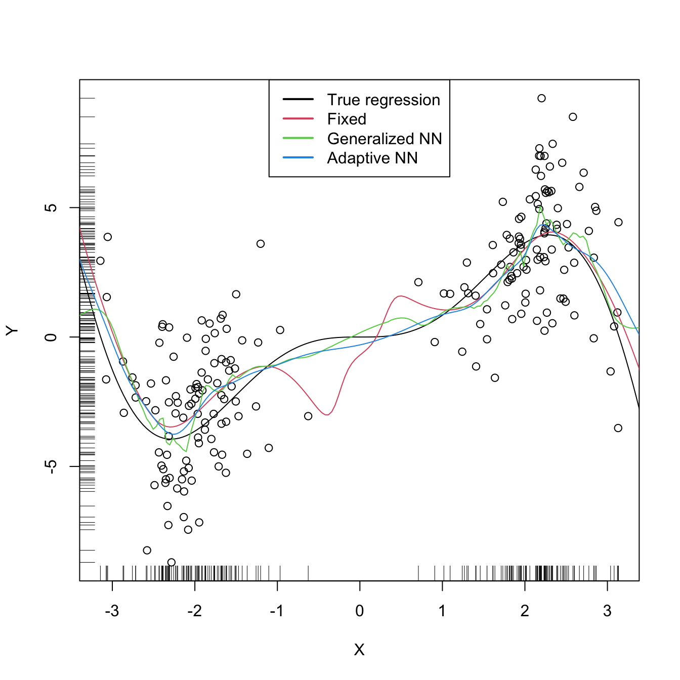

# Observe how the fixed bandwidth may yield a fit that produces serious
# artifacts in the low density region. At that region the NN-based bandwidths
# enlarge to borrow strength from the points in the high density regions,
# whereas in the high density regions they shrink to adapt faster to the
# changes of the regression function

References

Fan, J., and I. Gijbels. 1996. Local Polynomial Modelling and Its Applications. Vol. 66. Monographs on Statistics and Applied Probability. London: Chapman & Hall. https://doi.org/10.2307/2670134.

Nadaraya, E. A. 1964. “On Estimating Regression.” Teoriya Veroyatnostei i Ee Primeneniya 9 (1): 157–59. https://doi.org/10.1137/1109020.

Wand, M. P., and M. C. Jones. 1995. Kernel Smoothing. Vol. 60. Monographs on Statistics and Applied Probability. London: Chapman & Hall. https://doi.org/10.1007/978-1-4899-4493-1.

Watson, G. S. 1964. “Smooth Regression Analysis.” Sankhyā, Series A 26 (4): 359–72. https://www.jstor.org/stable/25049340.

---

203. Notice that it does not depend on $h_2,$ only on $h_1,$ the bandwidth employed for smoothing $X.$↩︎

204. Termed due to the coetaneous proposals by Nadaraya (1964) and Watson (1964).↩︎

205. Obviously, avoiding the spurious perfect fit attained with $\hat{m}(X_i):=Y_i,$ $i=1,\ldots,n.$↩︎

206. Here we employ $p$ for denoting the order of the Taylor expansion and, correspondingly, the order of the associated polynomial fit. Do not confuse $p$ with the number of original predictors for explaining $Y$ – there is only one predictor in this section, $X.$ However, with a local polynomial fit we expand this predictor to $p$ predictors based on $(X^1,X^2,\ldots,X^p).$↩︎

207. The rationale is simple: $(X_i,Y_i)$ should be more informative about $m(x)$ than $(X_j,Y_j)$ if $x$ and $X_i$ are closer than $x$ and $X_j.$ Observe that $Y_i$ and $Y_j$ are ignored in measuring this proximity.↩︎

208. Recall that weighted least squares already appeared in the IRLS of Section 5.2.2.↩︎

209. Recall that the entries of $\hat{\boldsymbol{\beta}}_h$ are estimating $\boldsymbol{\beta}=\left(m(x), m'(x),\frac{m'(x)}{2},\ldots,\frac{m^{(p)}(x)}{p!}\right)',$ so we are indeed estimating $m(x)$ (first entry) and, in addition, its derivatives up to order $p$!↩︎

210. The lowess estimator, related with loess, is the one employed in R’s panel.smooth, which is the function in charge of displaying the smooth fits in lm and glm regression diagnostics. For those diagnostics, it employs a prefixed and not data-driven smoothing span of $2/3$ – which makes it inevitably a bad choice for certain data patterns. An example of data pattern for which the span $2/3$ is not appropriate is the one in upper right panel in Figure 5.15.↩︎

211. We do not address the analysis of the general case in which $p\geq1.$ The reader is referred to, e.g., Theorem 3.1 of Fan and Gijbels (1996) for the full analysis.↩︎

212. Recall that these are the only assumptions done so far in the model! Compared with the ones made for linear models or generalized linear models, they are extremely mild.↩︎

213. This assumption requires certain smoothness of the regression function, allowing thus for Taylor expansions to be performed. This assumption is important in practice: $\hat{m}(\cdot;p,h)$ is infinitely differentiable if the considered kernels $K$ are.↩︎

214. Avoids the situation in which $Y$ is a degenerated random variable.↩︎

215. Avoids the degenerate situation in which $m$ is estimated at regions without observations of the predictors (such as holes in the support of $X$).↩︎

216. Meaning that there exist a positive lower bound for $f.$↩︎

217. Mild assumption inherited from the kde.↩︎

218. Key assumption for reducing the bias and variance of $\hat{m}(\cdot;p,h)$ simultaneously.↩︎

219. The notation $o_\mathbb{P}(a_n)$ stands for a random variable that converges in probability to zero at a rate faster than $a_n\to0.$ It is mostly employed for denoting non-important terms in asymptotic expansions, like the ones in (6.24)–(6.25).↩︎

220. Recall that this makes perfect sense: low density regions of $X$ imply less information about $m$ available.↩︎

221. The same happened in the the linear model with the error variance $\sigma^2.$↩︎

222. The variance of an unweighted mean is reduced by a factor $n^{-1}$ when $n$ observations are employed. For computing $\hat{m}(x;p,h),$ $n$ observations are used but in a weighted fashion that roughly amounts to considering $nh$ unweighted observations.↩︎

223. Further details are available in Section 5.8 of Wand and Jones (1995) and references therein.↩︎

224. A fit based on ordinal polynomial fits but done in different blocks of the data.↩︎

225. Recall that $h$ is a tuning parameter!↩︎

226. Indeed, for any other linear smoother of the response, the result also holds.↩︎