5.7 Model diagnostics
As it was implicit in Section 5.2, generalized linear models are built on some probabilistic assumptions that are required for performing inference on the model parameters \(\boldsymbol{\beta}\) and \(\phi.\)
In general, if we employ the canonical link function, we assume that the data has been generated from (independence is implicit)
\[\begin{align} Y&|(X_1=x_{1},\ldots,X_p=x_{p})\sim\mathrm{E}(\eta(x_1,\ldots,x_p),\phi,a,b,c),\tag{5.34} \end{align}\]
in such a way that
\[\begin{align*} \mu=\mathbb{E}[Y|X_1=x_{1},\ldots,X_p=x_{p}]=g^{-1}(\eta), \end{align*}\]
and \(\eta(x_1,\ldots,x_p)=\beta_0+\beta_1x_{1}+\cdots+\beta_px_{p}.\)
In the case of the logistic and Poisson regressions, both with canonical link functions, the general model takes the form (independence is implicit)
\[\begin{align} Y|(X_1=x_1,\ldots,X_p=x_p)&\sim\mathrm{Ber}\left(\mathrm{logistic}(\eta)\right), \tag{5.35}\\ Y|(X_1=x_1,\ldots,X_p=x_p)&\sim\mathrm{Pois}\left(e^{\eta}\right). \tag{5.36} \end{align}\]
The assumptions behind (5.34), (5.35), and (5.36) are:
- Linearity in the transformed expectation: \(\mathbb{E}[Y|X_1=x_1,\ldots,X_p=x_p]=g^{-1}\left(\beta_0+\beta_1x_1+\cdots+\beta_px_p\right).\)
- Response distribution: \(Y|\mathbf{X}=\mathbf{x}\sim\mathrm{E}(\eta(\mathbf{x}),\phi,a,b,c)\) (the scale \(\phi\) and the functions \(a,b,c\) are constant for \(\mathbf{x}\)).
- Independence: \(Y_1,\ldots,Y_n\) are independent, conditionally on \(\mathbf{X}_1,\ldots,\mathbf{X}_n.\)
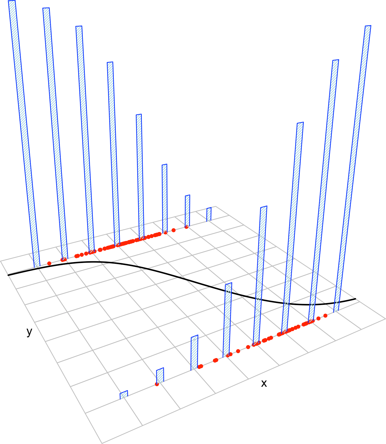
Figure 5.11: The key concepts of the logistic model. The red points represent a sample with population logistic curve \(y=\mathrm{logistic}(\beta_0+\beta_1x),\) shown in black. The blue bars represent the conditional probability mass functions of \(Y\) given \(X=x,\) whose means lie in the logistic curve.
There are two important points of the linear model assumptions “missing” here:
- Where is homoscedasticity? Homoscedasticity is specific to certain exponential family distributions in which \(\theta\) does not affect the variance. This is not the case for binomial or Poisson distributions variables, which result in heteroscedastic models. Also, homoscedasticity is the consequence of assumption ii in the case of the normal distribution.
- Where are the errors? The errors are not fundamental for building the linear model, but just a helpful concept related to least squares. The linear model can be constructed “without errors” directly using (2.8).
Recall that:
- Nothing is said about the distribution of \(X_1,\ldots,X_p.\) They could be deterministic or random. They could be discrete or continuous.
- \(X_1,\ldots,X_p\) are not required to be independent between them.
Checking the assumptions of a generalized linear model is more complicated than what we did in Section 3.5. The reason is the heterogeneity and heteroscedasticity of the responses, which makes the inspection of the residuals \(Y_i-\hat Y_i\) complicated.181 The first step is to construct some residuals \(\hat\varepsilon_i\) that are simpler to analyze.
The deviance residuals are the generalization of the residuals \(\hat\varepsilon_i=Y_i-\hat Y_i\) from the linear model. They are constructed using the analogy between the deviance and the RSS saw in (5.31). The deviance can be expressed into a sum of terms associated to each datum (recall, e.g., (5.30)):
\[\begin{align*} D=\sum_{i=1}^n d_i. \end{align*}\]
For the linear model, \(d_i=\hat\varepsilon_i^2,\) since \(D=\mathrm{RSS}(\hat{\boldsymbol{\beta}}).\) Based on this, we can define the deviance residuals as
\[\begin{align*} \hat\varepsilon_i^D:=\mathrm{sign}(Y_i-\hat \mu_i)\sqrt{d_i},\quad i=1,\ldots,n \end{align*}\]
and have a generalization of \(\hat\varepsilon_i\) for generalized linear models. This definition has interesting distributional consequences. From (5.32), we know that \(D^*\stackrel{a}{\sim}\chi_{n-p-1}^2.\) This suggests182 that
\[\begin{align} \hat\varepsilon_i^D\text{ are approximately normal if the model holds}.\tag{5.37} \end{align}\]
The previous statement is of variable accuracy, depending on the model, sample size, and distribution of the predictors.183 In the linear model, it is exact and \((\hat\varepsilon_1^D,\ldots,\hat\varepsilon_n^D)\) are distributed exactly as a \(\mathcal{N}_n(\mathbf{0},\sigma^2\mathbf{X}'(\mathbf{X}'\mathbf{X})^{-1}\mathbf{X}).\)
The deviance residuals are key for the diagnostics of generalized linear models. Whenever we refer to “residuals”, we understand that we refer to the deviance residuals (since several definitions of residuals are possible). They are also the residuals returned in R, either by glm$residuals or by residuals(glm).
The definition of the deviance residuals has interesting connections:
- If the canonical function is employed, then \(\sum_{i=1}^n \hat\varepsilon_i^D=0,\) as in the linear model.
- The estimate of the scale parameter can be seen as \(\hat\phi_D=\frac{\sum_{i=1}^n(\hat\varepsilon_i^D)^2}{n-p-1},\) which is perfectly coherent with \(\hat\sigma^2\) in the linear model.
- Therefore, \(\hat\phi_D\) is the sample variance of \(\hat\varepsilon_1^D,\ldots,\hat\varepsilon_n^D,\) which suggets that \(\phi\) is the asymptotic variance of the population deviance residuals, in other words, \(\mathbb{V}\mathrm{ar}[\varepsilon^D]\approx \phi.\)
- The deviance residuals equal the standard residuals in the linear model.
The script used for generating the following (perhaps surprising) Figures 5.12–5.23 is available here.
5.7.1 Linearity
Linearity between the transformed expectation of \(Y\) and the predictors \(X_1,\ldots,X_p\) is the building block of generalized linear models. If this assumption fails, then all the conclusions we might extract from the analysis are suspected to be flawed. Therefore it is a key assumption.
How to check it
We use the residuals vs. fitted values plot, which for generalized linear models is the scatterplot of \(\{(\hat{\eta}_i, \hat{\varepsilon}_i^D)\}_{i=1}^n.\) Recall that it is not the scatterplot of \(\{(\hat{Y}_i, \hat{\varepsilon}_i)\}_{i=1}^n.\) Under linearity, we expect that there is no trend in the residuals \(\hat\varepsilon_i^D\) with respect to \(\hat \eta_i,\) in addition to the patterns inherent to the nature of the response. If nonlinearities are observed, it is worth plotting the regression terms of the model via termplot.
What to do it fails
Using an adequate nonlinear transformation for the problematic predictors or adding interaction terms might be helpful. Alternatively, considering a nonlinear transformation \(f\) for the response \(Y\) might also be helpful, at expenses of the same comments given in Section 3.5.1.
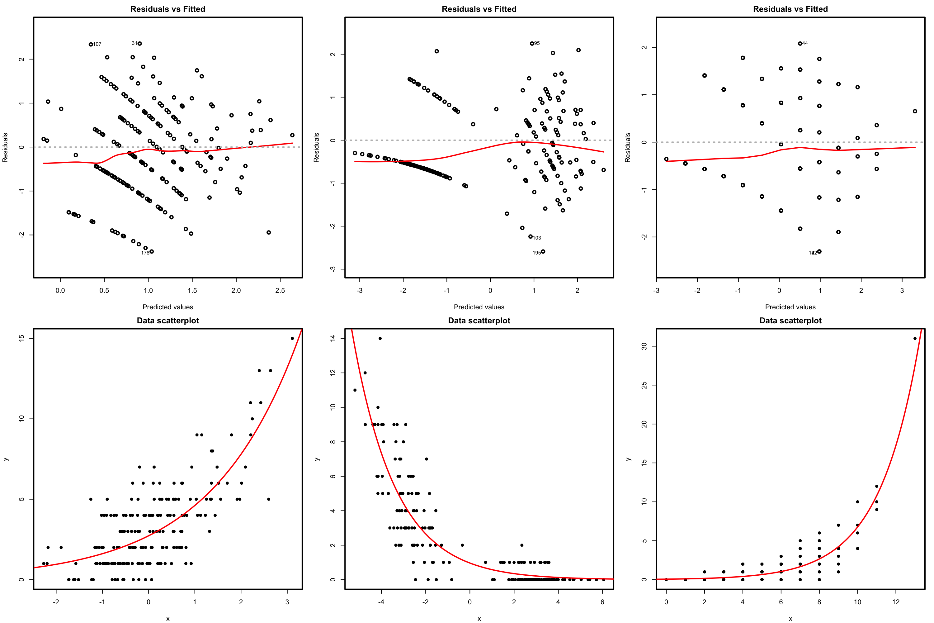
Figure 5.12: Residuals vs. fitted values plots (first row) for datasets (second row) respecting the linearity assumption in Poisson regression.
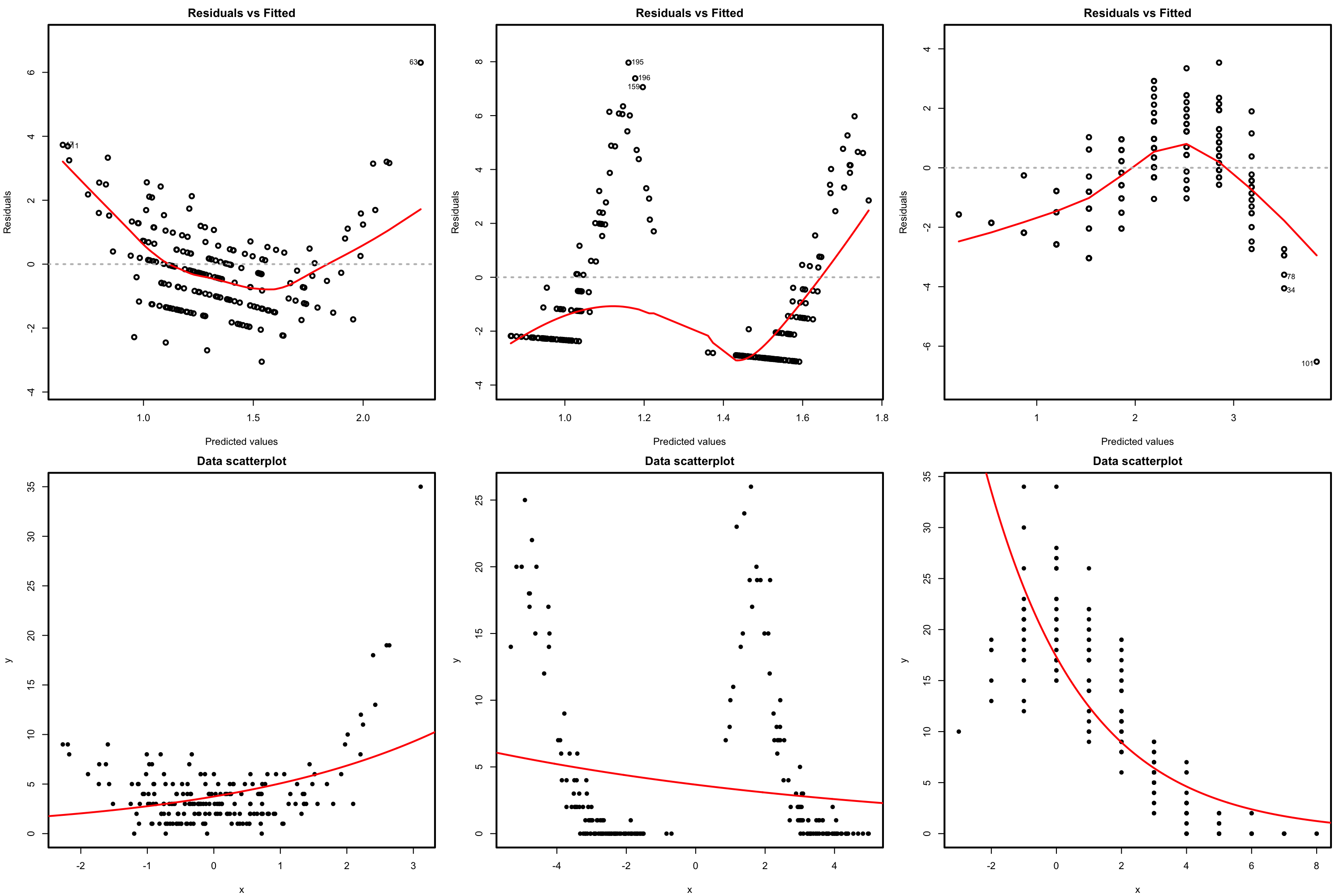
Figure 5.13: Residuals vs. fitted values plots (first row) for datasets (second row) violating the linearity assumption in Poisson regression.
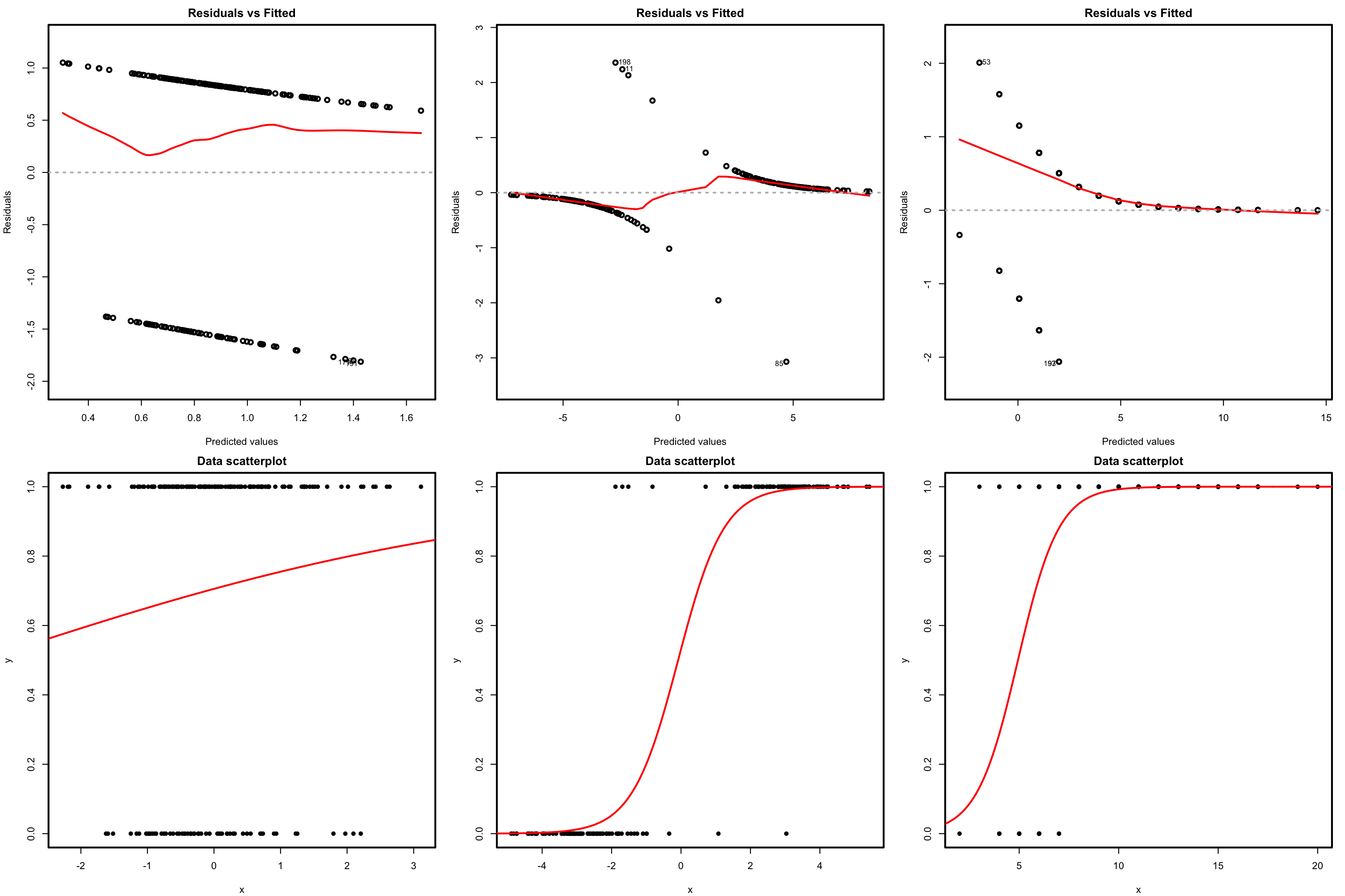
Figure 5.14: Residuals vs. fitted values plots (first row) for datasets (second row) respecting the linearity assumption in logistic regression.
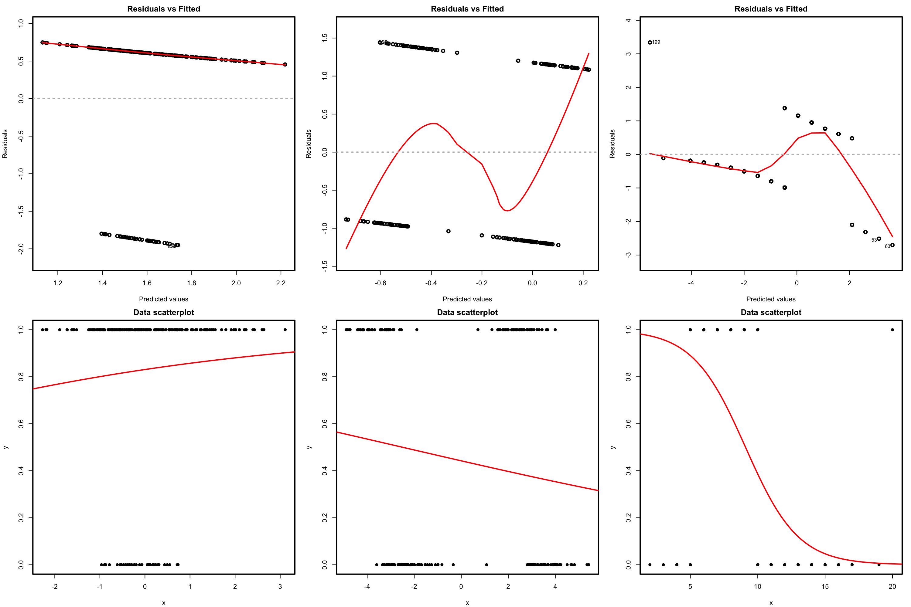
Figure 5.15: Residuals vs. fitted values plots (first row) for datasets (second row) violating the linearity assumption in logistic regression.
5.7.2 Response distribution
The approximate normality in the deviance residuals allows to evaluate how well satisfied the assumption of the response distribution is. The good news is that we can do so without relying on ad-hoc tools for each distribution.184 The bad news is that we have to pay an important price in terms of inexactness, since we employ an asymptotic distribution. The speed of this asymptotic convergence and the effective validity of (5.37) largely depends on several aspects: distribution of the response, sample size, and distribution of the predictors.
How to check it
The QQ-plot allows us to check if the standardized residuals follow a \(\mathcal{N}(0,1).\) Under the correct distribution of the response, we expect the points to align with the diagonal line. It is usual to have departures from the diagonal in the extremes other than in the center, even under normality, although these departures are more evident if the data is non normal. Unfortunately, it is also possible to have severe departures from normality even if the model is perfectly correct, see below. The reason is simply that the deviance residuals are significantly non-normal, which happens often in logistic regression.
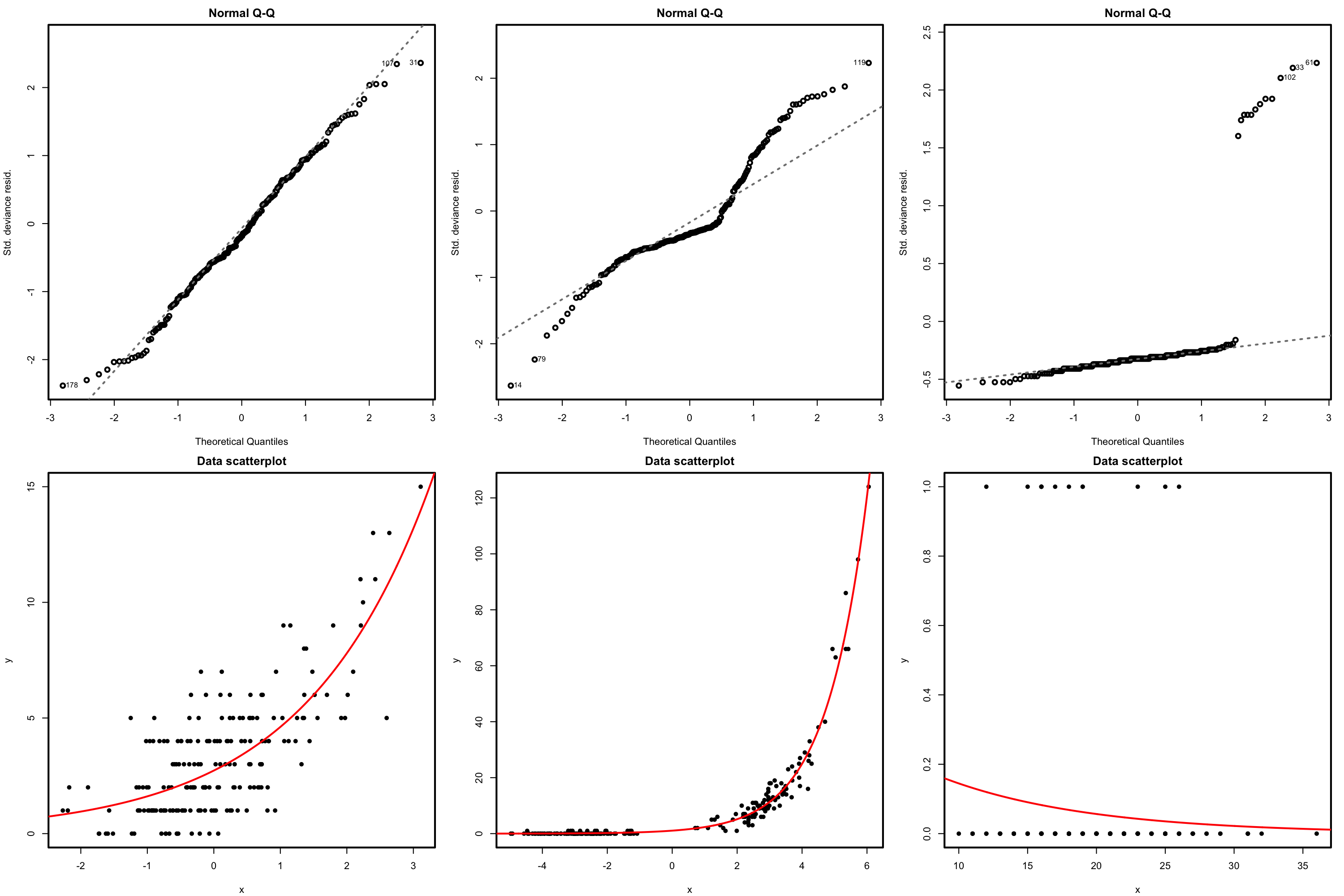
Figure 5.16: QQ-plots for the deviance residuals (first row) for datasets (second row) respecting the response distribution assumption for Poisson regression.
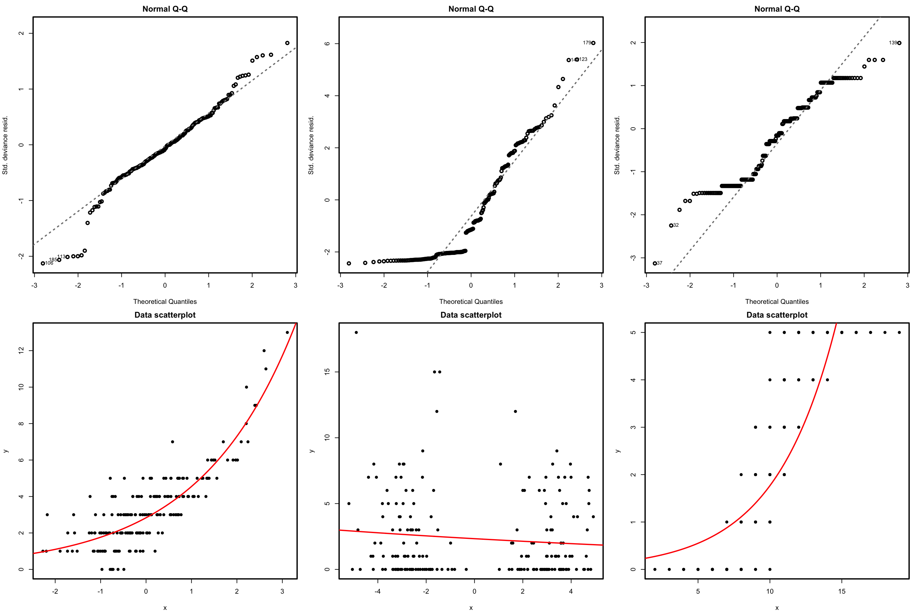
Figure 5.17: QQ-plots for the deviance residuals (first row) for datasets (second row) violating the response distribution assumption for Poisson regression.
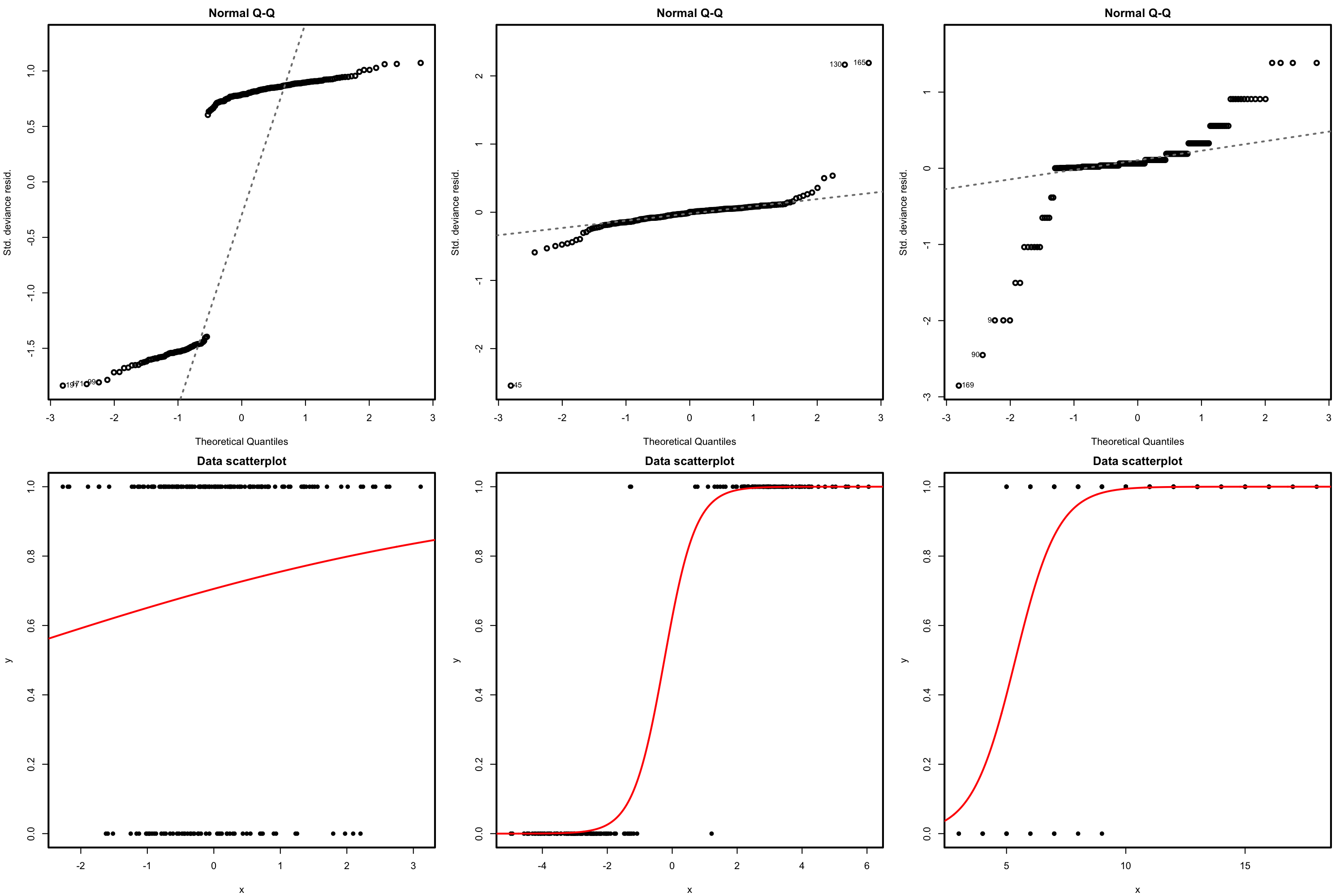
Figure 5.18: QQ-plots for the deviance residuals (first row) for datasets (second row) respecting the response distribution assumption for logistic regression.
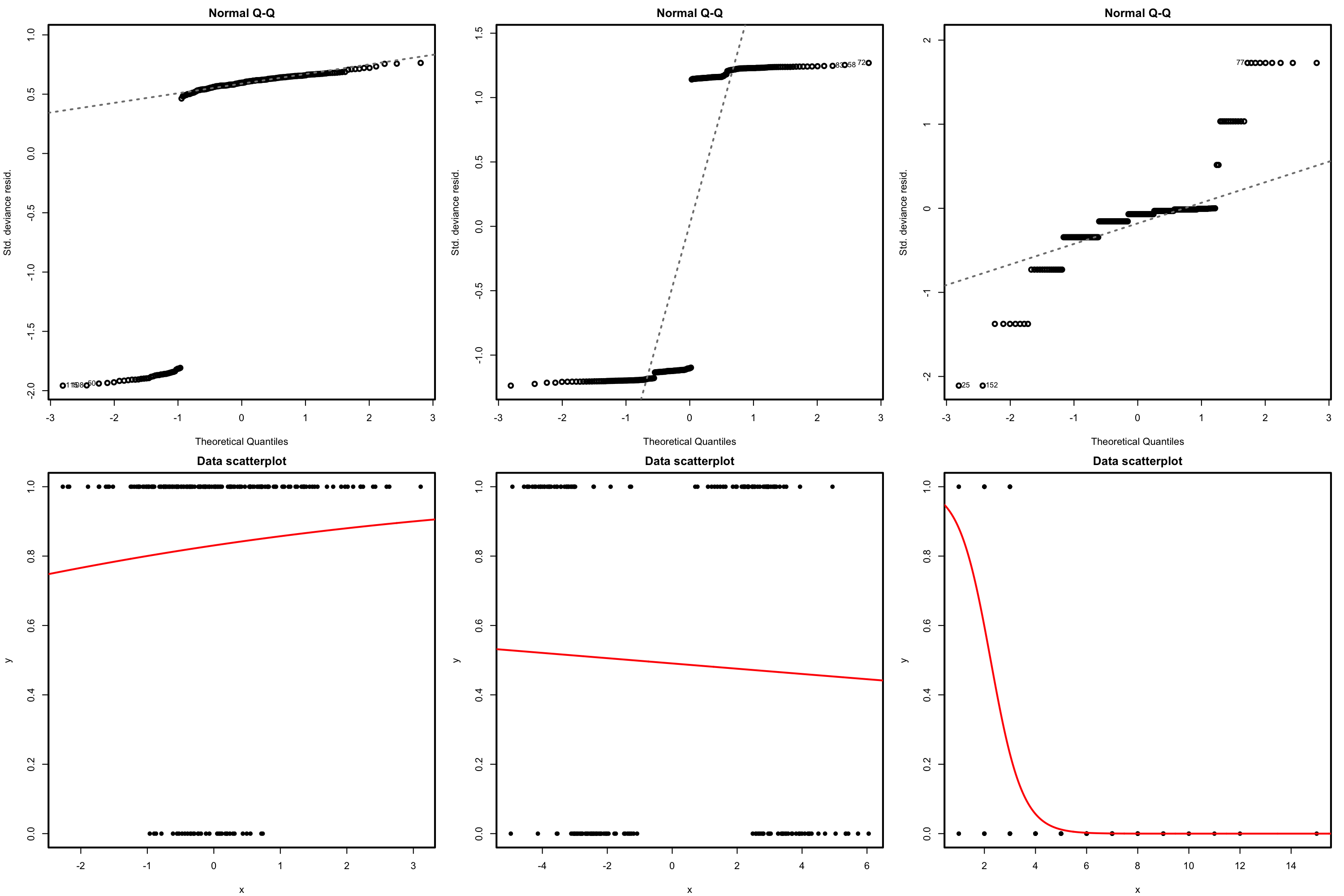
Figure 5.19: QQ-plots for the deviance residuals (first row) for datasets (second row) violating the response distribution assumption for logistic regression.
What to do it fails
Patching the distribution assumption is not easy and requires the consideration of more flexible models. One possibility is to transform \(Y\) by means of one of the transformations discussed in Section 3.5.2, of course at the price of modeling the transformed response rather than \(Y.\)
5.7.3 Independence
Independence is also a key assumption: it guarantees that the amount of information that we have on the relationship between \(Y\) and \(X_1,\ldots,X_p\) with \(n\) observations is maximal.
How to check it
The presence of autocorrelation in the residuals can be examined by means of a serial plot of the residuals. Under uncorrelation, we expect the series to show no tracking of the residuals, which is a sign of positive serial correlation. Negative serial correlation can be identified in the form of a small-large or positive-negative systematic alternation of the residuals. This can be explored better with lag.plot, as saw in Section 3.5.4.
What to do it fails
As in the linear model, little can be done if there is dependence in the data, once this has been collected. If serial dependence is present, a differentiation of the response may lead to independent observations.
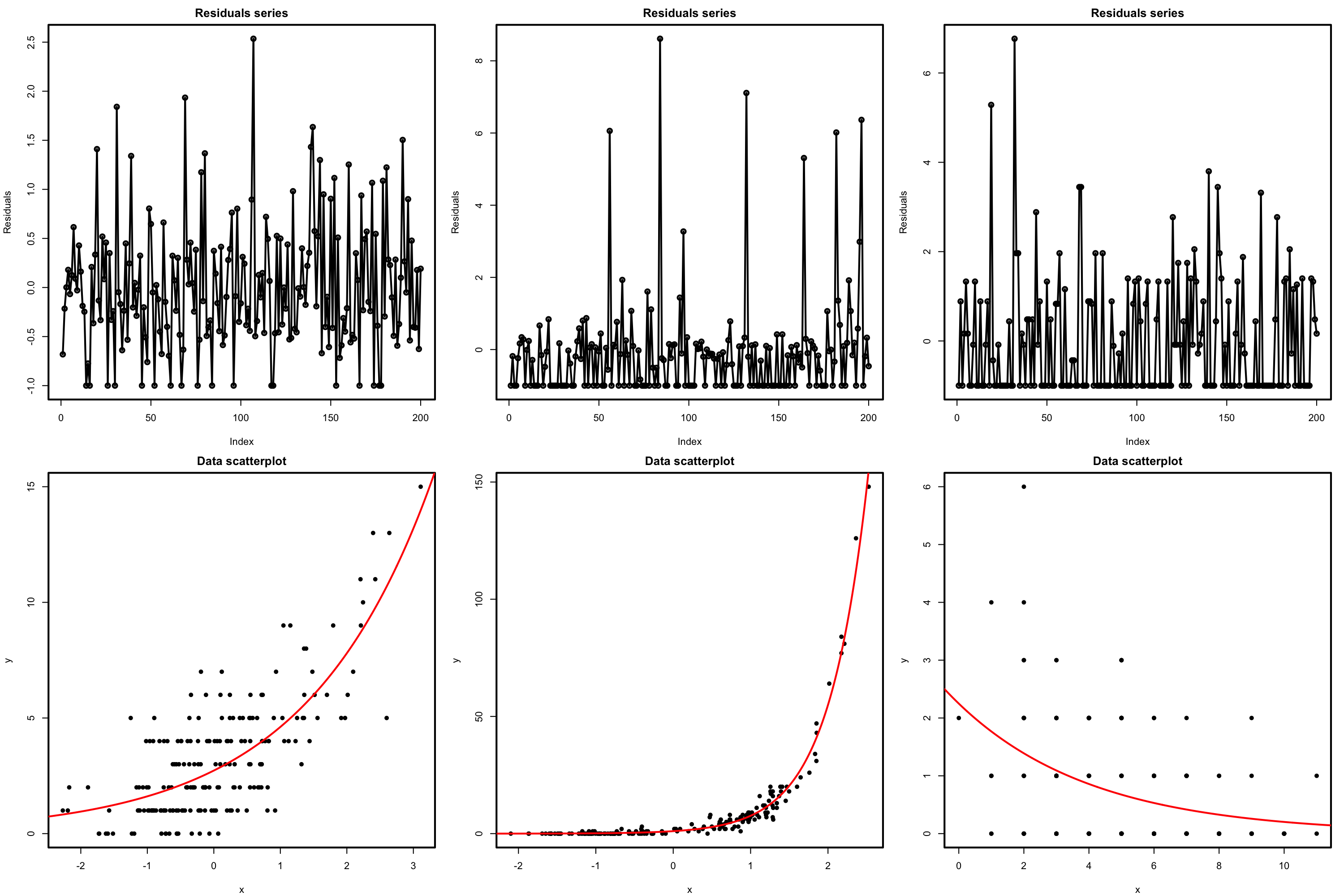
Figure 5.20: Serial plots of the residuals (first row) for datasets (second row) respecting the independence assumption for Poisson regression.
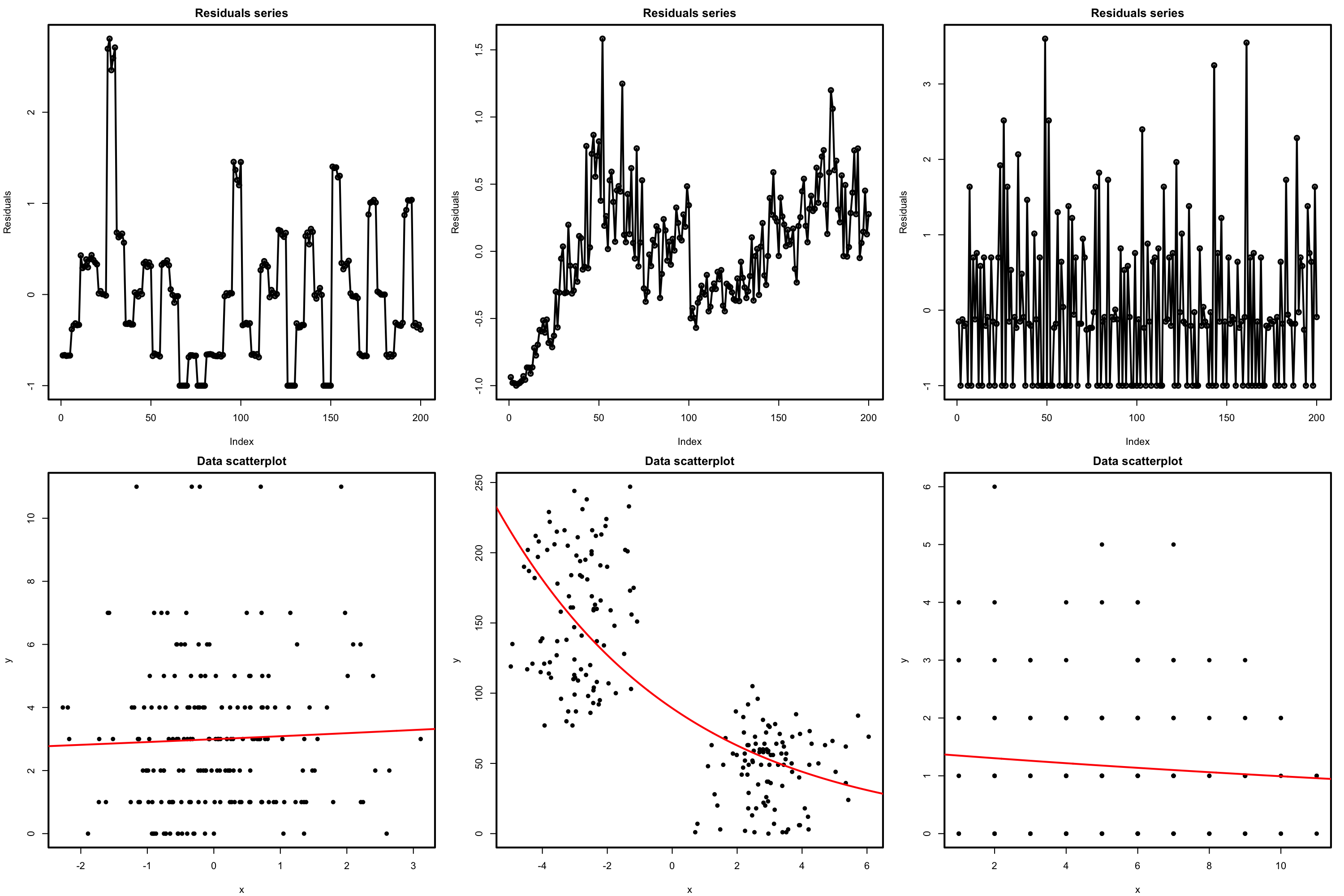
Figure 5.21: Serial plots of the residuals (first row) for datasets (second row) violating the independence assumption for Poisson regression.
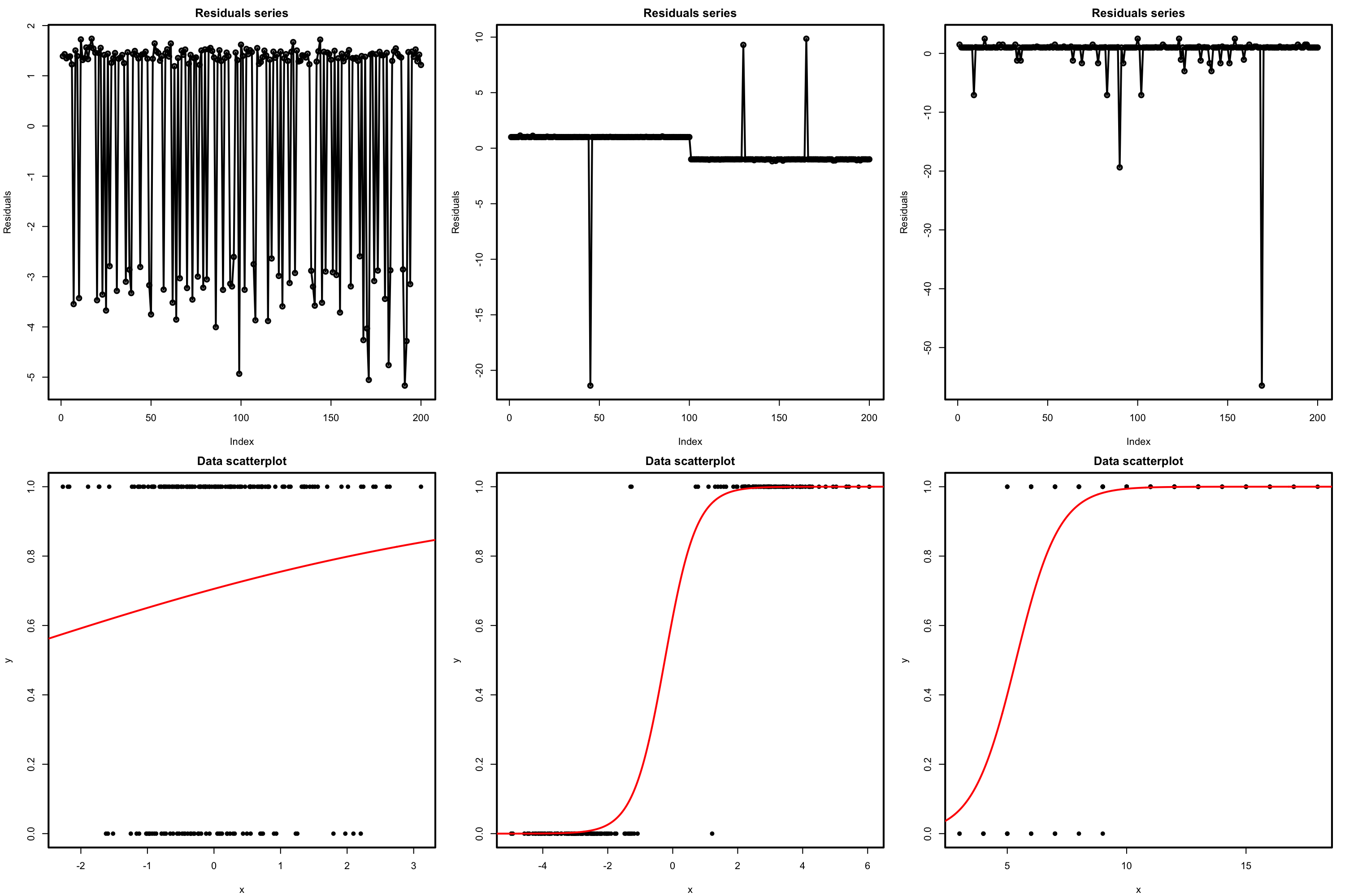
Figure 5.22: Serial plots of the residuals (first row) for datasets (second row) respecting the independence assumption for logistic regression.
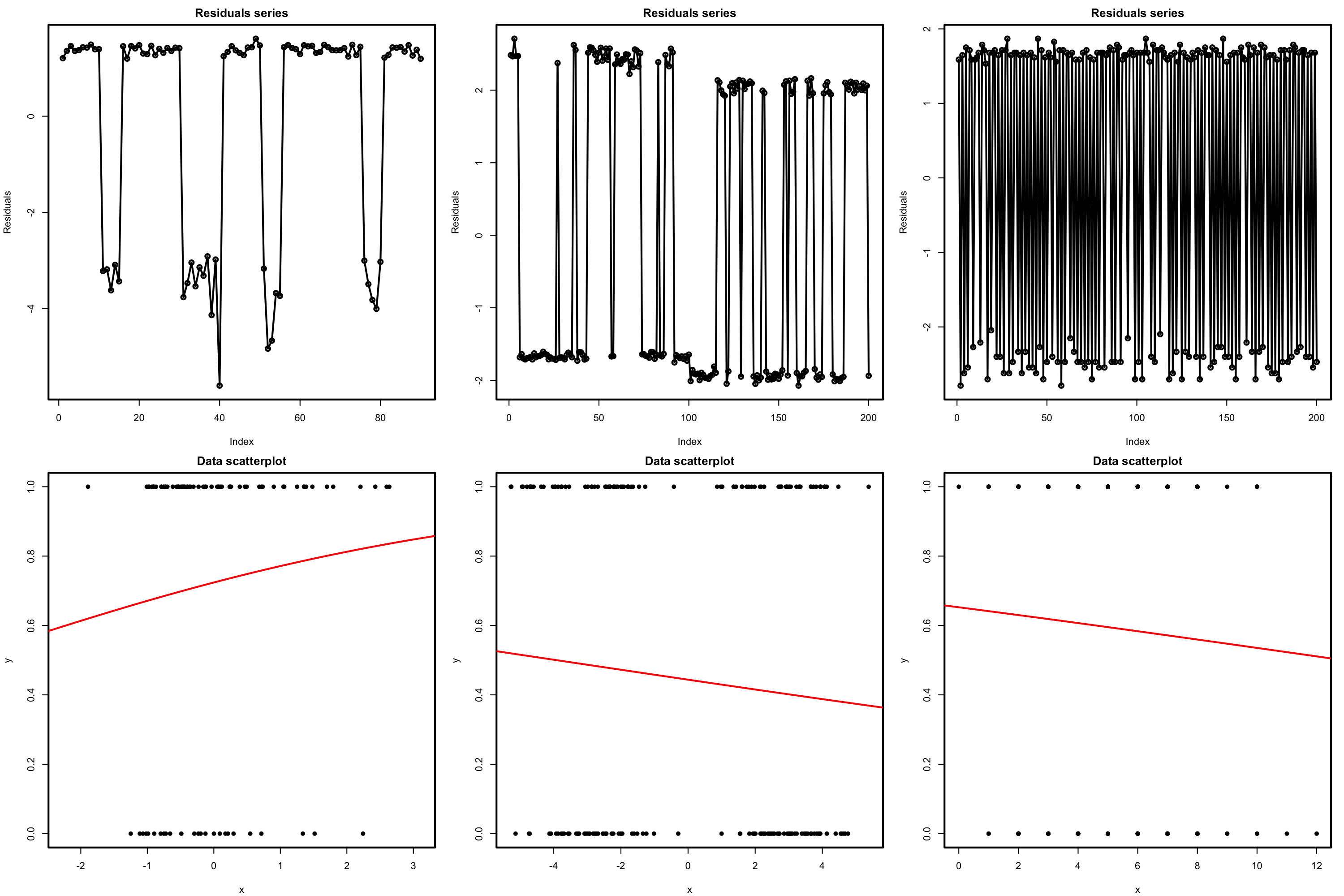
Figure 5.23: Serial plots of the residuals (first row) for datasets (second row) violating the independence assumption for logistic regression.
5.7.4 Multicollinearity
Multicollinearity can also be present in generalized linear models. Despite the nonlinear effect of the predictors on the response, the predictors are combined linearly in (5.4). Due to this, if two or more predictors are highly correlated between them, the fit of the model will be compromised since the individual linear effect of each predictor will be hard to separate from the rest of correlated predictors.
Then, a useful way of detecting multicollinearity is to inspect the VIF of each coefficient. The situation is exactly the same as in linear regression, since VIF looks only into the linear relations of the predictors. Therefore, the rule of thumb is the same as in Section 3.5.5:
- VIF close to 1: absence of multicollinearity.
- VIF larger than 5 or 10: problematic amount of multicollinearity. Advised to remove the predictor with largest VIF.
# Create predictors with multicollinearity: x4 depends on the rest
set.seed(45678)
x1 <- rnorm(100)
x2 <- 0.5 * x1 + rnorm(100)
x3 <- 0.5 * x2 + rnorm(100)
x4 <- -x1 + x2 + rnorm(100, sd = 0.25)

# Response
z <- 1 + 0.5 * x1 + 2 * x2 - 3 * x3 - x4
y <- rbinom(n = 100, size = 1, prob = 1/(1 + exp(-z)))
data <- data.frame(x1 = x1, x2 = x2, x3 = x3, x4 = x4, y = y)

# Correlations -- none seems suspicious
cor(data)
##            x1         x2         x3         x4           y
## x1  1.0000000 0.38254782  0.2142011 -0.5261464  0.20198825
## x2  0.3825478 1.00000000  0.5167341  0.5673174  0.07456324
## x3  0.2142011 0.51673408  1.0000000  0.2500123 -0.49853746
## x4 -0.5261464 0.56731738  0.2500123  1.0000000 -0.11188657
## y   0.2019882 0.07456324 -0.4985375 -0.1118866  1.00000000

# Abnormal generalized variance inflation factors: largest for x4, we remove it
modMultiCo <- glm(y ~ x1 + x2 + x3 + x4, family = "binomial")
car::vif(modMultiCo)
##       x1       x2       x3       x4
## 27.84756 36.66514  4.94499 36.78817

# Without x4
modClean <- glm(y ~ x1 + x2 + x3, family = "binomial")

# Comparison
summary(modMultiCo)
##
## Call:
## glm(formula = y ~ x1 + x2 + x3 + x4, family = "binomial")
##
## Deviance Residuals:
##     Min       1Q   Median       3Q      Max
## -2.4743  -0.3796   0.1129   0.4052   2.3887
##
## Coefficients:
##             Estimate Std. Error z value Pr(>|z|)
## (Intercept)   1.2527     0.4008   3.125  0.00178 **
## x1           -3.4269     1.8225  -1.880  0.06007 .
## x2            6.9627     2.1937   3.174  0.00150 **
## x3           -4.3688     0.9312  -4.691 2.71e-06 ***
## x4           -5.0047     1.9440  -2.574  0.01004 *
## ---
## Signif. codes:  0 '***' 0.001 '**' 0.01 '*' 0.05 '.' 0.1 ' ' 1
##
## (Dispersion parameter for binomial family taken to be 1)
##
##     Null deviance: 132.81  on 99  degrees of freedom
## Residual deviance:  59.76  on 95  degrees of freedom
## AIC: 69.76
##
## Number of Fisher Scoring iterations: 7
summary(modClean)
##
## Call:
## glm(formula = y ~ x1 + x2 + x3, family = "binomial")
##
## Deviance Residuals:
##     Min       1Q   Median       3Q      Max
## -2.0952  -0.4144   0.1839   0.4762   2.5736
##
## Coefficients:
##             Estimate Std. Error z value Pr(>|z|)
## (Intercept)   0.9237     0.3221   2.868 0.004133 **
## x1            1.2803     0.4235   3.023 0.002502 **
## x2            1.7946     0.5290   3.392 0.000693 ***
## x3           -3.4838     0.7491  -4.651 3.31e-06 ***
## ---
## Signif. codes:  0 '***' 0.001 '**' 0.01 '*' 0.05 '.' 0.1 ' ' 1
##
## (Dispersion parameter for binomial family taken to be 1)
##
##     Null deviance: 132.813  on 99  degrees of freedom
## Residual deviance:  68.028  on 96  degrees of freedom
## AIC: 76.028
##
## Number of Fisher Scoring iterations: 6

# Generalized variance inflation factors normal
car::vif(modClean)
##       x1       x2       x3
## 1.674300 2.724351 3.743940Also, due to the variety of ranges the response \(Y\) is allowed to take in generalized linear models.↩︎
The logic behind the statement is that a \(\chi^2_k\) random variable has the same distribution as the sum of \(k\) independent squared \(\mathcal{N}(0,1)\) variables.↩︎
Practical counterexamples to the statement are possible, see Figures 5.16 and 5.18.↩︎
This would be the rigorous approach, but it is notably more complex.↩︎