4.3 Multivariate multiple linear model
So far, we have been interested in predicting/explaining a single response \(Y\) from a set of predictors \(X_1,\ldots,X_p.\) However, we might want to predict/explain several responses \(Y_1,\ldots,Y_q.\)133 As we will see, the model construction and estimation are quite analogous to the univariate multiple linear model, yet more cumbersome in notation.
4.3.1 Model formulation and least squares
The centered134 population version of the multivariate multiple linear model is
\[\begin{align*} Y_1&=\beta_{11}X_1+\cdots+\beta_{p1}X_p+\varepsilon_1, \\ & \vdots\\ Y_q&=\beta_{1q}X_1+\cdots+\beta_{pq}X_p+\varepsilon_q, \end{align*}\]
or, equivalently in matrix form,
\[\begin{align} \mathbf{Y}=\mathbf{B}'\mathbf{X}+\boldsymbol{\varepsilon}\tag{4.17} \end{align}\]
where \(\boldsymbol{\varepsilon}:=(\varepsilon_1,\ldots,\varepsilon_q)'\) is a random vector with null expectation, \(\mathbf{Y}=(Y_1,\ldots,Y_q)'\) and \(\mathbf{X}=(X_1,\ldots,X_p)'\) are random vectors, and
\[\begin{align*} \mathbf{B}=\begin{pmatrix} \beta_{11} & \ldots & \beta_{1q} \\ \vdots & \ddots & \vdots \\ \beta_{p1} & \ldots & \beta_{pq} \end{pmatrix}_{p\times q}. \end{align*}\]
Clearly, this construction implies that the conditional expectation of the random vector \(\mathbf{Y}\) is
\[\begin{align*} \mathbb{E}[\mathbf{Y}|\mathbf{X}=\mathbf{x}]=\mathbf{B}'\mathbf{x}. \end{align*}\]
Given a sample \(\{(\mathbf{X}_i,\mathbf{Y}_i)\}_{i=1}^n\) of observations of \((X_1,\ldots,X_p)\) and \((Y_1,\ldots,Y_q),\) the sample version of (4.17) is
\[\begin{align} \begin{pmatrix} Y_{11} & \ldots & Y_{1q} \\ \vdots & \ddots & \vdots \\ Y_{n1} & \ldots & Y_{nq} \end{pmatrix}_{n\times q}\!\!\! &= \begin{pmatrix} X_{11} & \ldots & X_{1p} \\ \vdots & \ddots & \vdots \\ X_{n1} & \ldots & X_{np} \end{pmatrix}_{n\times p} \begin{pmatrix} \beta_{11} & \ldots & \beta_{1q} \\ \vdots & \ddots & \vdots \\ \beta_{p1} & \ldots & \beta_{pq} \end{pmatrix}_{p\times q}\!\!\! + \begin{pmatrix} \varepsilon_{11} & \ldots & \varepsilon_{1q} \\ \vdots & \ddots & \vdots \\ \varepsilon_{n1} & \ldots & \varepsilon_{nq} \end{pmatrix}_{n\times q},\tag{4.18} \end{align}\]
or, equivalently in matrix form,
\[\begin{align} \mathbb{Y}=\mathbb{X}\mathbf{B}+\mathbf{E},\tag{4.19} \end{align}\]
where \(\mathbb{Y},\) \(\mathbb{X},\) and \(\mathbf{E}\) are clearly identified by comparing (4.19) with (4.18).135
The approach for estimating \(\mathbf{B}\) is really similar to the univariate multiple linear model: minimize the sum of squared distances between the responses \(\mathbf{Y}_1,\ldots,\mathbf{Y}_n\) and their explanations \(\mathbf{B}'\mathbf{X}_1,\ldots,\mathbf{B}'\mathbf{X}_n.\) These distances are now measured by the \(\|\cdot\|_2\) norm in \(\mathbb{R}^q,\) resulting
\[\begin{align*} \mathrm{RSS}(\mathbf{B})&:=\sum_{i=1}^n\|\mathbf{Y}_i-\mathbf{B}'\mathbf{X}_i\|^2_2\\ &=\sum_{i=1}^n(\mathbf{Y}_i-\mathbf{B}'\mathbf{X}_i)'(\mathbf{Y}_i-\mathbf{B}'\mathbf{X}_i)\\ &=\mathrm{tr}\left((\mathbb{Y}-\mathbb{X}\mathbf{B})'(\mathbb{Y}-\mathbb{X}\mathbf{B})\right). \end{align*}\]
The similarities with (2.6) are clear and it is immediate to see that (2.6) appears as a special case136 for \(q=1.\) The minimizer of \(\mathrm{RSS}(\mathbf{B})\) is obtained analogously to how the least squares estimator was obtained when \(q=1\):
\[\begin{align} \hat{\mathbf{B}}&:=\arg\min_{\mathbf{B}\in\mathcal{M}_{p\times q}}\mathrm{RSS}(\mathbf{B})=(\mathbb{X}'\mathbb{X})^{-1}\mathbb{X}'\mathbb{Y}.\tag{4.20} \end{align}\]
Recall that if the responses and predictors are not centered, then the estimate of the intercept is simply obtained from the sample means \(\bar{\mathbf{Y}}:=(\bar Y_1,\ldots,\bar Y_q)'\) and \(\bar{\mathbf{X}}=(\bar X_1,\ldots,\bar X_p)'\):
\[\begin{align*} \hat{\boldsymbol{\beta}}_0=\bar{\mathbf{Y}}-\hat{\mathbf{B}}'\bar{\mathbf{X}}. \end{align*}\]
Equation (4.20) reveals that fitting a \(q\)-multivariate linear model amounts to fitting \(q\) univariate linear models separately! Indeed, recall that \(\mathbf{B}=(\boldsymbol{\beta}_1 \cdots \boldsymbol{\beta}_q),\) where the column vector \(\boldsymbol{\beta}_j\) represents the vector of coefficients of the \(j\)-th univariate linear model. Then, comparing (4.20) with (2.7) (where \(\mathbb{Y}\) consisted of a single column) and by block matrix multiplication, we can clearly see that \(\hat{\mathbf{B}}\) is just the concatenation of the columns of \(\hat{\boldsymbol{\beta}}_j,\) \(j=1,\ldots,q,\) i.e., \(\hat{\mathbf{B}}=(\hat{\boldsymbol{\beta}}_1 \cdots \hat{\boldsymbol{\beta}}_q).\)
As happened in the univariate linear model, if \(p>n\) then the inverse of \(\mathbb{X}'\mathbb{X}\) in (4.20) does not exist. In that case, one should either remove predictors or resort to a shrinkage method that avoids inverting \(\mathbb{X}'\mathbb{X}.\) It is interesting to note, though, that \(q\) has no effect on the feasibility of the fitting, only \(p\) does. In particular it is possible to compute (4.20) with \(q\gg n,\) and hence \(pq\gg n,\) i.e., the number of estimated parameters can be much larger than \(n\).
We see next how to do multivariate multiple linear regression in R with a simulated example.
# Dimensions and sample size
p <- 3
q <- 2
n <- 100

# A quick way of creating a non-diagonal (valid) covariance matrix for the
# errors
Sigma <- 3 * toeplitz(seq(1, 0.1, l = q))
set.seed(12345)
X <- mvtnorm::rmvnorm(n = n, mean = 1:p, sigma = diag(0.5, nrow = p, ncol = p))
E <- mvtnorm::rmvnorm(n = n, mean = rep(0, q), sigma = Sigma)

# Linear model
B <- matrix((-1)^(1:p) * (1:p), nrow = p, ncol = q, byrow = TRUE)
Y <- X %*% B + E

# Fitting the model (note: Y and X are matrices!)
mod <- lm(Y ~ X)
mod
##
## Call:
## lm(formula = Y ~ X)
##
## Coefficients:
##              [,1]      [,2]
## (Intercept)   0.05017  -0.36899
## X1           -0.54770   2.06905
## X2           -3.01547  -0.78308
## X3            1.88327  -3.00840
# Note that the intercept is markedly different from zero -- that is because
# X is not centered

# Compare with B
B
##      [,1] [,2]
## [1,]   -1    2
## [2,]   -3   -1
## [3,]    2   -3

# Summary of the model: gives q separate summaries, one for each fitted
# univariate model
summary(mod)
## Response Y1 :
##
## Call:
## lm(formula = Y1 ~ X)
##
## Residuals:
##     Min      1Q  Median      3Q     Max
## -4.0432 -1.3513  0.2592  1.1325  3.5298
##
## Coefficients:
##             Estimate Std. Error t value Pr(>|t|)
## (Intercept)  0.05017    0.96251   0.052   0.9585
## X1          -0.54770    0.24034  -2.279   0.0249 *
## X2          -3.01547    0.26146 -11.533  < 2e-16 ***
## X3           1.88327    0.21537   8.745 7.38e-14 ***
## ---
## Signif. codes:  0 '***' 0.001 '**' 0.01 '*' 0.05 '.' 0.1 ' ' 1
##
## Residual standard error: 1.695 on 96 degrees of freedom
## Multiple R-squared:  0.7033, Adjusted R-squared:  0.694
## F-statistic: 75.85 on 3 and 96 DF,  p-value: < 2.2e-16
##
##
## Response Y2 :
##
## Call:
## lm(formula = Y2 ~ X)
##
## Residuals:
##     Min      1Q  Median      3Q     Max
## -4.1385 -0.7922 -0.0486  0.8987  3.6599
##
## Coefficients:
##             Estimate Std. Error t value Pr(>|t|)
## (Intercept)  -0.3690     0.8897  -0.415  0.67926
## X1            2.0691     0.2222   9.314 4.44e-15 ***
## X2           -0.7831     0.2417  -3.240  0.00164 **
## X3           -3.0084     0.1991 -15.112  < 2e-16 ***
## ---
## Signif. codes:  0 '***' 0.001 '**' 0.01 '*' 0.05 '.' 0.1 ' ' 1
##
## Residual standard error: 1.567 on 96 degrees of freedom
## Multiple R-squared:  0.7868, Adjusted R-squared:  0.7801
## F-statistic: 118.1 on 3 and 96 DF,  p-value: < 2.2e-16

# Exactly equivalent to
summary(lm(Y[, 1] ~ X))
##
## Call:
## lm(formula = Y[, 1] ~ X)
##
## Residuals:
##     Min      1Q  Median      3Q     Max
## -4.0432 -1.3513  0.2592  1.1325  3.5298
##
## Coefficients:
##             Estimate Std. Error t value Pr(>|t|)
## (Intercept)  0.05017    0.96251   0.052   0.9585
## X1          -0.54770    0.24034  -2.279   0.0249 *
## X2          -3.01547    0.26146 -11.533  < 2e-16 ***
## X3           1.88327    0.21537   8.745 7.38e-14 ***
## ---
## Signif. codes:  0 '***' 0.001 '**' 0.01 '*' 0.05 '.' 0.1 ' ' 1
##
## Residual standard error: 1.695 on 96 degrees of freedom
## Multiple R-squared:  0.7033, Adjusted R-squared:  0.694
## F-statistic: 75.85 on 3 and 96 DF,  p-value: < 2.2e-16
summary(lm(Y[, 2] ~ X))
##
## Call:
## lm(formula = Y[, 2] ~ X)
##
## Residuals:
##     Min      1Q  Median      3Q     Max
## -4.1385 -0.7922 -0.0486  0.8987  3.6599
##
## Coefficients:
##             Estimate Std. Error t value Pr(>|t|)
## (Intercept)  -0.3690     0.8897  -0.415  0.67926
## X1            2.0691     0.2222   9.314 4.44e-15 ***
## X2           -0.7831     0.2417  -3.240  0.00164 **
## X3           -3.0084     0.1991 -15.112  < 2e-16 ***
## ---
## Signif. codes:  0 '***' 0.001 '**' 0.01 '*' 0.05 '.' 0.1 ' ' 1
##
## Residual standard error: 1.567 on 96 degrees of freedom
## Multiple R-squared:  0.7868, Adjusted R-squared:  0.7801
## F-statistic: 118.1 on 3 and 96 DF,  p-value: < 2.2e-16
Let’s see another quick example using the iris dataset.
# When we want to add several variables of a dataset as responses through a
# formula interface, we have to use cbind() in the response. Doing
# "Petal.Width + Petal.Length ~ ..." is INCORRECT, as lm will understand
# "I(Petal.Width + Petal.Length) ~ ..." and do one single regression

# Predict Petal's measurements from Sepal's
modIris <- lm(cbind(Petal.Width, Petal.Length) ~
                Sepal.Length + Sepal.Width + Species, data = iris)
summary(modIris)
## Response Petal.Width :
##
## Call:
## lm(formula = Petal.Width ~ Sepal.Length + Sepal.Width + Species,
##     data = iris)
##
## Residuals:
##      Min       1Q   Median       3Q      Max
## -0.50805 -0.10042 -0.01221  0.11416  0.46455
##
## Coefficients:
##                   Estimate Std. Error t value Pr(>|t|)
## (Intercept)       -0.86897    0.16985  -5.116 9.73e-07 ***
## Sepal.Length       0.06360    0.03395   1.873    0.063 .
## Sepal.Width        0.23237    0.05145   4.516 1.29e-05 ***
## Speciesversicolor  1.17375    0.06758  17.367  < 2e-16 ***
## Speciesvirginica   1.78487    0.07779  22.944  < 2e-16 ***
## ---
## Signif. codes:  0 '***' 0.001 '**' 0.01 '*' 0.05 '.' 0.1 ' ' 1
##
## Residual standard error: 0.1797 on 145 degrees of freedom
## Multiple R-squared:  0.9459, Adjusted R-squared:  0.9444
## F-statistic: 634.3 on 4 and 145 DF,  p-value: < 2.2e-16
##
##
## Response Petal.Length :
##
## Call:
## lm(formula = Petal.Length ~ Sepal.Length + Sepal.Width + Species,
##     data = iris)
##
## Residuals:
##      Min       1Q   Median       3Q      Max
## -0.75196 -0.18755  0.00432  0.16965  0.79580
##
## Coefficients:
##                   Estimate Std. Error t value Pr(>|t|)
## (Intercept)       -1.63430    0.26783  -6.102 9.08e-09 ***
## Sepal.Length       0.64631    0.05353  12.073  < 2e-16 ***
## Sepal.Width       -0.04058    0.08113  -0.500    0.618
## Speciesversicolor  2.17023    0.10657  20.364  < 2e-16 ***
## Speciesvirginica   3.04911    0.12267  24.857  < 2e-16 ***
## ---
## Signif. codes:  0 '***' 0.001 '**' 0.01 '*' 0.05 '.' 0.1 ' ' 1
##
## Residual standard error: 0.2833 on 145 degrees of freedom
## Multiple R-squared:  0.9749, Adjusted R-squared:  0.9742
## F-statistic:  1410 on 4 and 145 DF,  p-value: < 2.2e-16

# The fitted values and residuals are now matrices
head(modIris$fitted.values)
##   Petal.Width Petal.Length
## 1   0.2687095     1.519831
## 2   0.1398033     1.410862
## 3   0.1735565     1.273483
## 4   0.1439590     1.212910
## 5   0.2855861     1.451142
## 6   0.3807391     1.697490
head(modIris$residuals)
##   Petal.Width Petal.Length
## 1 -0.06870951 -0.119831001
## 2  0.06019672 -0.010861533
## 3  0.02644348  0.026517420
## 4  0.05604099  0.287089900
## 5 -0.08558613 -0.051141525
## 6  0.01926089  0.002510054

# The individual models
modIris1 <- lm(Petal.Width ~Sepal.Length + Sepal.Width + Species, data = iris)
modIris2 <- lm(Petal.Length ~Sepal.Length + Sepal.Width + Species, data = iris)
summary(modIris1)
##
## Call:
## lm(formula = Petal.Width ~ Sepal.Length + Sepal.Width + Species,
##     data = iris)
##
## Residuals:
##      Min       1Q   Median       3Q      Max
## -0.50805 -0.10042 -0.01221  0.11416  0.46455
##
## Coefficients:
##                   Estimate Std. Error t value Pr(>|t|)
## (Intercept)       -0.86897    0.16985  -5.116 9.73e-07 ***
## Sepal.Length       0.06360    0.03395   1.873    0.063 .
## Sepal.Width        0.23237    0.05145   4.516 1.29e-05 ***
## Speciesversicolor  1.17375    0.06758  17.367  < 2e-16 ***
## Speciesvirginica   1.78487    0.07779  22.944  < 2e-16 ***
## ---
## Signif. codes:  0 '***' 0.001 '**' 0.01 '*' 0.05 '.' 0.1 ' ' 1
##
## Residual standard error: 0.1797 on 145 degrees of freedom
## Multiple R-squared:  0.9459, Adjusted R-squared:  0.9444
## F-statistic: 634.3 on 4 and 145 DF,  p-value: < 2.2e-16
summary(modIris2)
##
## Call:
## lm(formula = Petal.Length ~ Sepal.Length + Sepal.Width + Species,
##     data = iris)
##
## Residuals:
##      Min       1Q   Median       3Q      Max
## -0.75196 -0.18755  0.00432  0.16965  0.79580
##
## Coefficients:
##                   Estimate Std. Error t value Pr(>|t|)
## (Intercept)       -1.63430    0.26783  -6.102 9.08e-09 ***
## Sepal.Length       0.64631    0.05353  12.073  < 2e-16 ***
## Sepal.Width       -0.04058    0.08113  -0.500    0.618
## Speciesversicolor  2.17023    0.10657  20.364  < 2e-16 ***
## Speciesvirginica   3.04911    0.12267  24.857  < 2e-16 ***
## ---
## Signif. codes:  0 '***' 0.001 '**' 0.01 '*' 0.05 '.' 0.1 ' ' 1
##
## Residual standard error: 0.2833 on 145 degrees of freedom
## Multiple R-squared:  0.9749, Adjusted R-squared:  0.9742
## F-statistic:  1410 on 4 and 145 DF,  p-value: < 2.2e-16
4.3.2 Assumptions and inference
As deduced from what we have seen so far, fitting a multivariate linear regression is more practical than doing \(q\) separate univariate fits (especially if the number of responses \(q\) is large). However, it is not conceptually different. The discussion becomes more interesting in the inference for the multivariate linear regression, where the dependence between the responses has to be taken into account.
In order to achieve inference, we will require some assumptions, these being natural extensions of the ones seen in Section 2.3:
- Linearity: \(\mathbb{E}[\mathbf{Y}|\mathbf{X}=\mathbf{x}]=\mathbf{B}'\mathbf{x}.\)
- Homoscedasticity: \(\mathbb{V}\text{ar}[\boldsymbol{\varepsilon}|X_1=x_1,\ldots,X_p=x_p]=\boldsymbol{\Sigma}.\)
- Normality: \(\boldsymbol{\varepsilon}\sim\mathcal{N}_q(\mathbf{0},\boldsymbol{\Sigma}).\)
- Independence of the errors: \(\boldsymbol{\varepsilon}_1,\ldots,\boldsymbol{\varepsilon}_n\) are independent (or uncorrelated, \(\mathbb{E}[\boldsymbol{\varepsilon}_i\boldsymbol{\varepsilon}_j']=\mathbf{0},\) \(i\neq j,\) since they are assumed to be normal).
Then, a good one-line summary of the multivariate multiple linear model is (independence is implicit)
\[\begin{align*} \mathbf{Y}|\mathbf{X}=\mathbf{x}\sim \mathcal{N}_q(\mathbf{B}'\mathbf{x},\boldsymbol{\Sigma}). \end{align*}\]
Based on these assumptions, the key result for rooting inference is the distribution of \(\hat{\mathbf{B}}=(\hat{\boldsymbol{\beta}}_1 \cdots \hat{\boldsymbol{\beta}}_q)\) as an estimator of \(\mathbf{B}=(\boldsymbol{\beta}_1 \cdots \boldsymbol{\beta}_q).\) This result is now more cumbersome,137 but we can state it as
\[\begin{align} \hat{\boldsymbol{\beta}}_j&\sim\mathcal{N}_{p}\left(\boldsymbol{\beta}_j,\sigma_j^2(\mathbb{X}'\mathbb{X})^{-1}\right),\quad j=1,\ldots,q,\tag{4.21}\\ \begin{pmatrix} \hat{\boldsymbol{\beta}}_j\\ \hat{\boldsymbol{\beta}}_k \end{pmatrix}&\sim\mathcal{N}_{2p}\left(\begin{pmatrix} \boldsymbol{\beta}_j\\ \boldsymbol{\beta}_k \end{pmatrix}, \begin{pmatrix} \sigma_{j}^2(\mathbb{X}'\mathbb{X})^{-1} & \sigma_{jk}(\mathbb{X}'\mathbb{X})^{-1} \\ \sigma_{jk}(\mathbb{X}'\mathbb{X})^{-1} & \sigma_{k}^2(\mathbb{X}'\mathbb{X})^{-1} \end{pmatrix} \right),\quad j,k=1,\ldots,q,\tag{4.22} \end{align}\]
where \(\boldsymbol\Sigma=(\sigma_{ij})\) and \(\sigma_{ii}=\sigma_{i}^2.\)138
The results (4.21)–(4.22) open the way for obtaining hypothesis tests on the joint significance of a predictor in the model (for the \(q\) responses, not just for one), confidence intervals for the coefficients, prediction confidence regions for the conditional expectation and the conditional response, the Multivariate ANOVA (MANOVA) decomposition, multivariate extensions of the \(F\)-test, and others. However, due to the correlation between responses and the multivariateness, these inferential tools are more complex than in the univariate linear model. Therefore, given the increased complexity, we do not go into more details and refer the interested reader to, e.g., Chapter 8 in Seber (1984). We illustrate with code, though, the most important practical aspects.
# Confidence intervals for the parameters
confint(modIris)
##                                       2.5 %     97.5 %
## Petal.Width:(Intercept)        -1.204674903 -0.5332662
## Petal.Width:Sepal.Length       -0.003496659  0.1307056
## Petal.Width:Sepal.Width         0.130680383  0.3340610
## Petal.Width:Speciesversicolor   1.040169583  1.3073259
## Petal.Width:Speciesvirginica    1.631118293  1.9386298
## Petal.Length:(Intercept)       -2.163654566 -1.1049484
## Petal.Length:Sepal.Length       0.540501864  0.7521177
## Petal.Length:Sepal.Width       -0.200934599  0.1197646
## Petal.Length:Speciesversicolor  1.959595164  2.3808588
## Petal.Length:Speciesvirginica   2.806663658  3.2915610
# Warning! Do not confuse Petal.Width:Sepal.Length with an interaction term!
# It is meant to represent the Response:Predictor coefficient

# Prediction -- now more limited without confidence intervals implemented
predict(modIris, newdata = iris[1:3, ])
##   Petal.Width Petal.Length
## 1   0.2687095     1.519831
## 2   0.1398033     1.410862
## 3   0.1735565     1.273483

# MANOVA table
manova(modIris)
## Call:
##    manova(modIris)
##
## Terms:
##                 Sepal.Length Sepal.Width  Species Residuals
## Petal.Width          57.9177      6.3975  17.5745    4.6802
## Petal.Length        352.8662     50.0224  49.7997   11.6371
## Deg. of Freedom            1           1        2       145
##
## Residual standard errors: 0.1796591 0.2832942
## Estimated effects may be unbalanced

# "Same" as the "Sum Sq" and "Df" entries of
anova(modIris1)
## Analysis of Variance Table
##
## Response: Petal.Width
##               Df Sum Sq Mean Sq F value    Pr(>F)
## Sepal.Length   1 57.918  57.918 1794.37 < 2.2e-16 ***
## Sepal.Width    1  6.398   6.398  198.21 < 2.2e-16 ***
## Species        2 17.574   8.787  272.24 < 2.2e-16 ***
## Residuals    145  4.680   0.032
## ---
## Signif. codes:  0 '***' 0.001 '**' 0.01 '*' 0.05 '.' 0.1 ' ' 1
anova(modIris2)
## Analysis of Variance Table
##
## Response: Petal.Length
##               Df Sum Sq Mean Sq F value    Pr(>F)
## Sepal.Length   1 352.87  352.87 4396.78 < 2.2e-16 ***
## Sepal.Width    1  50.02   50.02  623.29 < 2.2e-16 ***
## Species        2  49.80   24.90  310.26 < 2.2e-16 ***
## Residuals    145  11.64    0.08
## ---
## Signif. codes:  0 '***' 0.001 '**' 0.01 '*' 0.05 '.' 0.1 ' ' 1

# anova() serves for assessing the significance of including a new predictor
# for explaining all the responses. This is based on an extension of the
# *sequential* ANOVA table briefly covered in Section 2.6. The hypothesis test
# is by default conducted with the Pillai statistic (an extension of the F-test)
anova(modIris)
## Analysis of Variance Table
##
##               Df  Pillai approx F num Df den Df    Pr(>F)
## (Intercept)    1 0.99463  13332.6      2    144 < 2.2e-16 ***
## Sepal.Length   1 0.97030   2351.9      2    144 < 2.2e-16 ***
## Sepal.Width    1 0.81703    321.5      2    144 < 2.2e-16 ***
## Species        2 0.89573     58.8      4    290 < 2.2e-16 ***
## Residuals    145
## ---
## Signif. codes:  0 '***' 0.001 '**' 0.01 '*' 0.05 '.' 0.1 ' ' 1
4.3.3 Shrinkage
Applying shrinkage is also possible in multivariate linear models. In particular, this allows to fit models with \(p\gg n\) predictors.
The glmnet package implements the elastic net regularization for multivariate linear models. It features extensions of the \(\|\cdot\|_1\) and \(\|\cdot\|_2\) norm penalties for a vector of parameters in \(\mathbb{R}^p,\) as considered in Section 4.1, to norms for a matrix of parameters of size \(p\times q.\) Precisely:
- The ridge penalty \(\|\boldsymbol\beta_{-1}\|_2^2\) extends to \(\|\mathbf{B}\|_{\mathrm{F}}^2,\) where \(\|\mathbf{B}\|_{\mathrm{F}}=\sqrt{\sum_{i=1}^p\sum_{j=1}^q\beta_{ij}^2}\) is the Frobenius norm of \(\mathbf{B}.\) This is a global penalty to shrink \(\mathbf{B}.\)
- The lasso penalty \(\|\boldsymbol\beta_{-1}\|_1\) extends139 to \(\sum_{j=1}^p\|\mathbf{B}_j\|_2,\) where \(\mathbf{B}_j\) is the \(j\)-th row of \(\mathbf{B}.\) This is a rowwise penalty that seeks to effectively remove rows of \(\mathbf{B},\) thus eliminating predictors.140
Taking these two extensions into account, the elastic net loss is defined as:
\[\begin{align} \text{RSS}(\mathbf{B})+\lambda\left(\alpha\sum_{j=1}^p\|\mathbf{B}_j\|_2+(1-\alpha)\|\mathbf{B}\|_{\mathrm{F}}^2\right).\tag{4.23} \end{align}\]
Clearly, ridge regression corresponds to \(\alpha=0\) (quadratic penalty) and lasso to \(\alpha=1\) (rowwise penalty). And if \(\lambda=0,\) we are back to the least squares problem and theory. The optimization of (4.23) gives
\[\begin{align*} \hat{\mathbf{B}}_{\lambda,\alpha}:=\arg\min_{\mathbf{B}\in\mathcal{M}_{p\times q}}\left\{ \text{RSS}(\mathbf{B})+\lambda\left(\alpha\sum_{j=1}^p\|\mathbf{B}_j\|_2+(1-\alpha)\|\mathbf{B}\|_{\mathrm{F}}^2\right)\right\}. \end{align*}\]
From here, the workflow is very similar to the univariate linear model: we have to be aware that an standardization of \(\mathbb{X}\) and \(\mathbb{Y}\) takes place in glmnet; there are explicit formulas for the ridge regression estimator, but not for lasso; tuning parameter selection of \(\lambda\) is done by \(k\)-fold cross-validation and its one standard error variant; variable selection (zeroing of rows in \(\mathbf{B}\)) can be done with lasso.
The following chunk of code illustrates some of these points using glmnet::glmnet with family = "mgaussian" (do not forget this argument!).
# Simulate data
n <- 500
p <- 50
q <- 10
set.seed(123456)
X <- mvtnorm::rmvnorm(n = n, mean = p:1, sigma = 5 * 0.5^toeplitz(1:p))
E <- mvtnorm::rmvnorm(n = n, mean = rep(0, q), sigma = toeplitz(q:1))
B <- 5 * (2 / (0.5 * (1:p - 15)^2 + 2) + 1 / (0.1 * (1:p - 40)^2 + 1)) %*%
  t(1 / sqrt(1:q))
Y <- X %*% B + E

# Visualize B -- dark violet is close to 0
image(1:q, 1:p, t(B), col = viridisLite::viridis(20), xlab = "q", ylab = "p")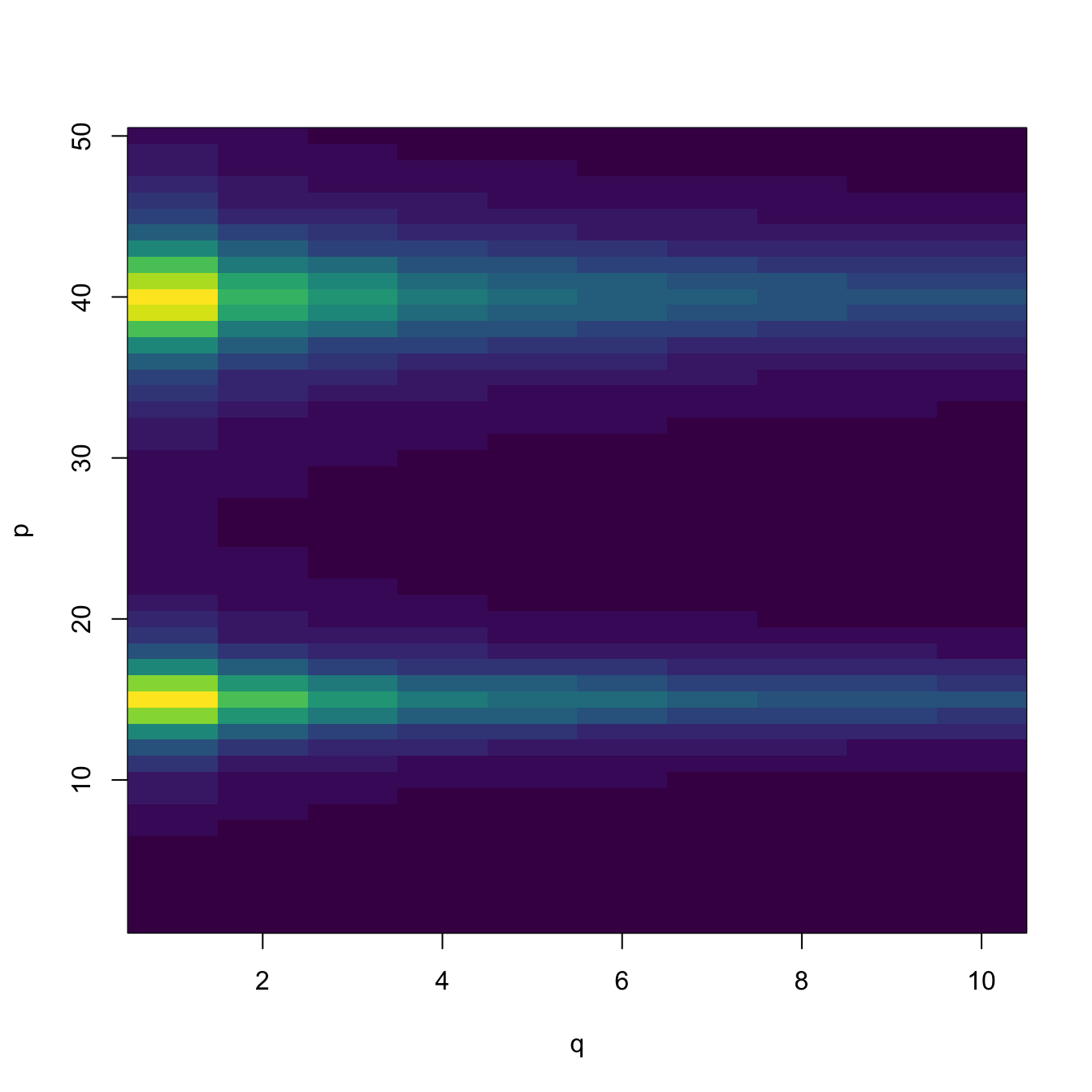
# Lasso path fit
mfit <- glmnet(x = X, y = Y, family = "mgaussian", alpha = 1)

# A list of models for each response
str(mfit$beta, 1)
## List of 10
##  $ y1 :Formal class 'dgCMatrix' [package "Matrix"] with 6 slots
##  $ y2 :Formal class 'dgCMatrix' [package "Matrix"] with 6 slots
##  $ y3 :Formal class 'dgCMatrix' [package "Matrix"] with 6 slots
##  $ y4 :Formal class 'dgCMatrix' [package "Matrix"] with 6 slots
##  $ y5 :Formal class 'dgCMatrix' [package "Matrix"] with 6 slots
##  $ y6 :Formal class 'dgCMatrix' [package "Matrix"] with 6 slots
##  $ y7 :Formal class 'dgCMatrix' [package "Matrix"] with 6 slots
##  $ y8 :Formal class 'dgCMatrix' [package "Matrix"] with 6 slots
##  $ y9 :Formal class 'dgCMatrix' [package "Matrix"] with 6 slots
##  $ y10:Formal class 'dgCMatrix' [package "Matrix"] with 6 slots

# Tuning parameter selection by 10-fold cross-validation
set.seed(12345)
kcvLassoM <- cv.glmnet(x = X, y = Y, family = "mgaussian", alpha = 1)
kcvLassoM$lambda.min
## [1] 0.135243
kcvLassoM$lambda.1se
## [1] 0.497475

# Location of both optimal lambdas in the CV loss function
indMin <- which.min(kcvLassoM$cvm)
plot(kcvLassoM)
abline(h = kcvLassoM$cvm[indMin] + c(0, kcvLassoM$cvsd[indMin]))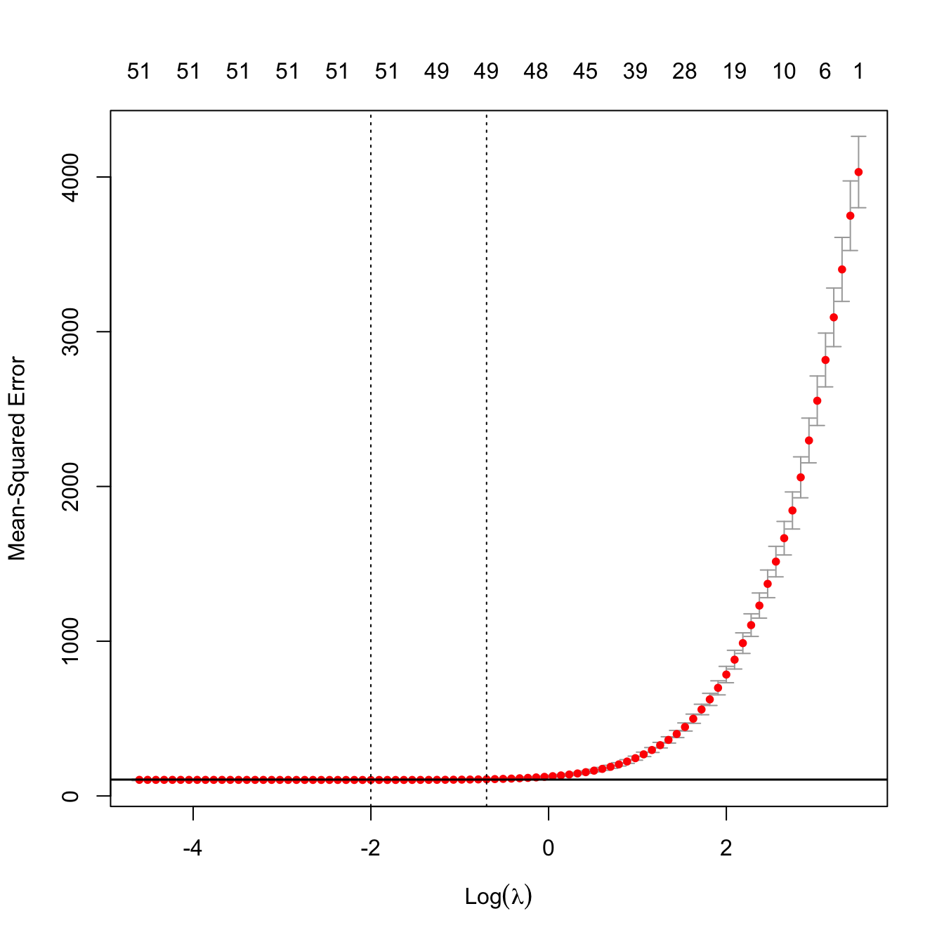
# Extract the coefficients associated to some fits
coefs <- predict(kcvLassoM, type = "coefficients",
                 s = c(kcvLassoM$lambda.min, kcvLassoM$lambda.1se))
str(coefs, 1)
## List of 10
##  $ y1 :Formal class 'dgCMatrix' [package "Matrix"] with 6 slots
##  $ y2 :Formal class 'dgCMatrix' [package "Matrix"] with 6 slots
##  $ y3 :Formal class 'dgCMatrix' [package "Matrix"] with 6 slots
##  $ y4 :Formal class 'dgCMatrix' [package "Matrix"] with 6 slots
##  $ y5 :Formal class 'dgCMatrix' [package "Matrix"] with 6 slots
##  $ y6 :Formal class 'dgCMatrix' [package "Matrix"] with 6 slots
##  $ y7 :Formal class 'dgCMatrix' [package "Matrix"] with 6 slots
##  $ y8 :Formal class 'dgCMatrix' [package "Matrix"] with 6 slots
##  $ y9 :Formal class 'dgCMatrix' [package "Matrix"] with 6 slots
##  $ y10:Formal class 'dgCMatrix' [package "Matrix"] with 6 slots

# Predictions for the first two observations
preds <- predict(kcvLassoM, type = "response",
                 s = c(kcvLassoM$lambda.min, kcvLassoM$lambda.1se),
                 newx = X[1:2, ])
preds
## , , 1
##
##            y1       y2       y3       y4       y5       y6       y7       y8       y9      y10
## [1,] 1607.532 1137.740 928.9553 804.5352 719.4861 656.1383 607.9023 568.9489 536.3892 508.3132
## [2,] 1598.747 1130.989 923.1741 799.3845 715.3698 652.8120 604.2244 565.1894 531.9679 504.8820
##
## , , 2
##
##            y1       y2       y3       y4       y5       y6       y7       y8       y9      y10
## [1,] 1606.685 1137.092 928.4553 804.0957 719.0616 655.7909 607.5870 568.5401 536.0135 508.0311
## [2,] 1600.321 1132.040 924.0621 800.1538 715.9371 653.3917 604.7983 565.6777 532.6244 505.4317
Finally, the next animation helps visualizing how the zeroing of the lasso happens for the estimator of \(\mathbf{B}\) with overall low absolute values on the previous simulated model.
manipulate::manipulate({

  # Color
  col <- viridisLite::viridis(20)

  # Common zlim
  zlim <- range(B) + c(-0.25, 0.25)

  # Plot true B
  par(mfrow = c(1, 2))
  image(1:q, 1:p, t(B), col = col, xlab = "q", ylab = "p", zlim = zlim,
        main = "B")

  # Extract B_hat from the lasso fit, a p x q matrix
  B_hat <- sapply(seq_along(mfit$beta), function(i) mfit$beta[i][[1]][, j])

  # Put as black rows the predictors included
  not_zero <- abs(B_hat) > 0
  image(1:q, 1:p, t(not_zero), breaks = c(0.5, 1),
        col = rgb(1, 1, 1, alpha = 0.1), add = TRUE)

  # For B_hat
  image(1:q, 1:p, t(B_hat), col = col, xlab = "q", ylab = "p", zlim = zlim,
        main = "Bhat")
  image(1:q, 1:p, t(not_zero), breaks = c(0.5, 1),
        col = rgb(1, 1, 1, alpha = 0.1), add = TRUE)

}, j = manipulate::slider(min = 1, max = ncol(mfit$beta$y1), step = 1,
                          label = "j in lambda(j)"))
References
Do not confuse them with \(Y_1,\ldots,Y_n,\) the notation employed in the rest of the sections for denoting the sample of the response \(Y.\)↩︎
Centering the responses and predictors is useful for removing the intercept term, allowing for simpler matricial versions.↩︎
The notation \(\mathbb{X}\) is introduced to avoid confusions between the design matrix \(\mathbb{X}\) and the random vector \(\mathbf{X}\) and observations \(\mathbf{X}_i,\) \(i=1,\ldots,n.\)↩︎
Employing the centered version of the univariate multiple linear model, as we have done in this section for the multivariate version.↩︎
Indeed, specifying the full distribution of \(\hat{\mathbf{B}}\) would require introducing the matrix normal distribution, a generalization of the \(p\)-dimensional normal seen in Section 1.3.↩︎
Observe how the covariance of the errors \(\varepsilon_j\) and \(\varepsilon_k,\) denoted by \(\sigma_{jk},\) is the responsible of the correlation between \(\hat{\boldsymbol{\beta}}_j\) and \(\hat{\boldsymbol{\beta}}_k\) in (4.22). If \(\sigma_{jk}=0,\) then \(\hat{\boldsymbol{\beta}}_j\) and \(\hat{\boldsymbol{\beta}}_k\) would be uncorrelated, thus independent because of their joint normality. Therefore, inference on \(\boldsymbol{\beta}_j\) and \(\boldsymbol{\beta}_k\) could be carried out separately.↩︎
If \(q=1,\) then \(\sum_{j=1}^p\|\mathbf{B}_j\|_2=\sum_{j=1}^p\sqrt{\beta_{j1}^2}=\sum_{j=1}^p|\beta_{j1}|.\)↩︎
This property would not hold if the penalty \(\sum_{i=1}^p\sum_{j=1}^q|\beta_{ij}|\) was considered.↩︎