2.2 Model formulation and least squares

In order to simplify the introduction of the foundations of the linear model, we first present the simple linear model and then extend it to the multiple linear model.

2.2.1 Simple linear model

The simple linear model is constructed by assuming that the linear relation

$\begin{align} Y = \beta_0 + \beta_1 X + \varepsilon \tag{2.1} \end{align}$

holds between $X$ and $Y.$ In (2.1), $\beta_0$ and $\beta_1$ are known as the intercept and slope, respectively. The random variable $\varepsilon$ has mean zero and is independent from $X.$ It describes the error around the mean, or the effect of other variables that we do not model. Another way of looking at (2.1) is

$\begin{align} \mathbb{E}[Y|X=x]=\beta_0+\beta_1x, \tag{2.2} \end{align}$

since $\mathbb{E}[\varepsilon|X=x]=0.$

The LHS of (2.2) is the conditional expectation of $Y$ given $X.$ It represents how the mean of the random variable $Y$ is changing according to a particular value $x$ of the random variable $X.$ With the RHS, what we are saying is that the mean of $Y$ is changing in a linear fashion with respect to the value of $X.$ Hence the clear interpretation of the coefficients:

$\beta_0$ : is the mean of $Y$ when $X=0.$
$\beta_1$ : is the increment in the mean of $Y$ for an increment of one unit in $X=x.$

If we have a sample $(X_1,Y_1),\ldots,(X_n,Y_n)$ for our random variables $X$ and $Y,$ we can estimate the unknown coefficients $\beta_0$ and $\beta_1.$ A possible way of doing so is by looking for certain optimality, for example the minimization of the Residual Sum of Squares (RSS):

$\begin{align*} \text{RSS}(\beta_0,\beta_1):=\sum_{i=1}^n(Y_i-\beta_0-\beta_1X_i)^2. \end{align*}$

In other words, we look for the estimators $(\hat\beta_0,\hat\beta_1)$ such that

$\begin{align*} (\hat\beta_0,\hat\beta_1)=\arg\min_{(\beta_0,\beta_1)\in\mathbb{R}^2} \text{RSS}(\beta_0,\beta_1). \end{align*}$

The motivation for minimizing the RSS is geometrical, as shown by Figure 2.3. We aim to minimize the squares of the distances of points projected vertically onto the line determined by $(\hat\beta_0,\hat\beta_1).$

Figure 2.3: The effect of the kind of distance in the error criterion. The choices of intercept and slope that minimize the sum of squared distances for one kind of distance are not the optimal choices for a different kind of distance. Application available here.

It can be seen that the minimizers of the RSS¹⁷ are

$\begin{align} \hat\beta_0=\bar{Y}-\hat\beta_1\bar{X},\quad \hat\beta_1=\frac{s_{xy}}{s_x^2},\tag{2.3} \end{align}$

where:

$\bar{X}=\frac{1}{n}\sum_{i=1}^nX_i$ is the sample mean.
$s_x^2=\frac{1}{n}\sum_{i=1}^n(X_i-\bar{X})^2$ is the sample variance.¹⁸
$s_{xy}=\frac{1}{n}\sum_{i=1}^n(X_i-\bar{X})(Y_i-\bar{Y})$ is the sample covariance. It measures the degree of linear association between $X_1,\ldots,X_n$ and $Y_1,\ldots,Y_n.$ Once scaled by $s_xs_y,$ it gives the sample correlation coefficient $r_{xy}=\frac{s_{xy}}{s_xs_y}.$

There are some important points hidden behind the election of RSS as the error criterion for obtaining $(\hat\beta_0,\hat\beta_1)$ :

Why the vertical distances and not horizontal or perpendicular? Because we want to minimize the error in the prediction of $Y$ ! Note that the treatment of the variables is not symmetrical.
Why the squares in the distances and not the absolute value? Due to mathematical convenience. Squares are nice to differentiate and are closely related with maximum likelihood estimation under the normal distribution (see Appendix A.2).

Let’s see how to obtain automatically the minimizers of the error in Figure 2.3 by the lm (linear model) function. The data of the figure has been generated with the following code:

# Generates 50 points from a N(0, 1): predictor and error
set.seed(34567)
x <- rnorm(n = 50)
eps <- rnorm(n = 50)

# Responses
yLin <- -0.5 + 1.5 * x + eps
yQua <- -0.5 + 1.5 * x^2 + eps
yExp <- -0.5 + 1.5 * 2^x + eps

# Data
leastSquares <- data.frame(x = x, yLin = yLin, yQua = yQua, yExp = yExp)

For a simple linear model, lm has the syntax lm(formula = response ~ predictor, data = data), where response and predictor are the names of two variables in the data frame data. Note that the LHS of ~ represents the response and the RHS the predictors.

# Call lm
lm(yLin ~ x, data = leastSquares)
## 
## Call:
## lm(formula = yLin ~ x, data = leastSquares)
## 
## Coefficients:
## (Intercept)            x  
##     -0.6154       1.3951
lm(yQua ~ x, data = leastSquares)
## 
## Call:
## lm(formula = yQua ~ x, data = leastSquares)
## 
## Coefficients:
## (Intercept)            x  
##      0.9710      -0.8035
lm(yExp ~ x, data = leastSquares)
## 
## Call:
## lm(formula = yExp ~ x, data = leastSquares)
## 
## Coefficients:
## (Intercept)            x  
##       1.270        1.007

# The lm object
mod <- lm(yLin ~ x, data = leastSquares)
mod
## 
## Call:
## lm(formula = yLin ~ x, data = leastSquares)
## 
## Coefficients:
## (Intercept)            x  
##     -0.6154       1.3951

# We can produce a plot with the linear fit easily
plot(x, yLin)
abline(coef = mod$coefficients, col = 2)

Figure 2.4: Linear fit for the data employed in Figure 2.3 minimizing the RSS.


# Access coefficients with $coefficients
mod$coefficients
## (Intercept)           x 
##  -0.6153744   1.3950973

# Compute the minimized RSS
sum((yLin - mod$coefficients[1] - mod$coefficients[2] * x)^2)
## [1] 41.02914
sum(mod$residuals^2)
## [1] 41.02914

# mod is a list of objects whose names are
names(mod)
##  [1] "coefficients"  "residuals"     "effects"       "rank"          "fitted.values" "assign"        "qr"           
##  [8] "df.residual"   "xlevels"       "call"          "terms"         "model"

Check that you can not improve the error in Figure 2.3 when using the coefficients given by lm, if vertical distances are selected. Check also that these coefficients are only optimal for vertical distances.

An interesting exercise is to check that lm is actually implementing the estimates given in (2.3):

# Covariance
Sxy <- cov(x, yLin)

# Variance
Sx2 <- var(x)

# Coefficients
beta1 <- Sxy / Sx2
beta0 <- mean(yLin) - beta1 * mean(x)
c(beta0, beta1)
## [1] -0.6153744  1.3950973

# Output from lm
mod <- lm(yLin ~ x, data = leastSquares)
mod$coefficients
## (Intercept)           x 
##  -0.6153744   1.3950973

The population regression coefficients, $(\beta_0,\beta_1),$ are not the same as the estimated regression coefficients, $(\hat\beta_0,\hat\beta_1)$ :

$(\beta_0,\beta_1)$ are the theoretical and always unknown quantities (except under controlled scenarios).
$(\hat\beta_0,\hat\beta_1)$ are the estimates computed from the data. They are random variables, since they are computed from the random sample $(X_1,Y_1),\ldots,(X_n,Y_n).$

In an abuse of notation, the term regression line is often used to denote both the theoretical ( $y=\beta_0+\beta_1x$ ) and the estimated ( $y=\hat\beta_0+\hat\beta_1x$ ) regression lines.

2.2.2 Case study application

Let’s get back to the wine dataset and compute some simple linear regressions. Prior to that, let’s begin by summarizing the information in Table 2.1 to get a grasp of the structure of the data. For that, we first correctly import the dataset into R:

# Read data
wine <- read.table(file = "wine.csv", header = TRUE, sep = ",")

Now we can conduct a quick exploratory analysis to have insights into the data:

# Numerical -- marginal distributions
summary(wine)
##       Year          Price         WinterRain         AGST        HarvestRain         Age          FrancePop    
##  Min.   :1952   Min.   :6.205   Min.   :376.0   Min.   :14.98   Min.   : 38.0   Min.   : 3.00   Min.   :43184  
##  1st Qu.:1960   1st Qu.:6.508   1st Qu.:543.5   1st Qu.:16.15   1st Qu.: 88.0   1st Qu.: 9.50   1st Qu.:46856  
##  Median :1967   Median :6.984   Median :600.0   Median :16.42   Median :123.0   Median :16.00   Median :50650  
##  Mean   :1967   Mean   :7.042   Mean   :608.4   Mean   :16.48   Mean   :144.8   Mean   :16.19   Mean   :50085  
##  3rd Qu.:1974   3rd Qu.:7.441   3rd Qu.:705.5   3rd Qu.:17.01   3rd Qu.:185.5   3rd Qu.:22.50   3rd Qu.:53511  
##  Max.   :1980   Max.   :8.494   Max.   :830.0   Max.   :17.65   Max.   :292.0   Max.   :31.00   Max.   :55110

# Graphical -- pairwise relations with linear and "smooth" regressions
car::scatterplotMatrix(wine, col = 1, regLine = list(col = 2),
                       smooth = list(col.smooth = 4, col.spread = 4))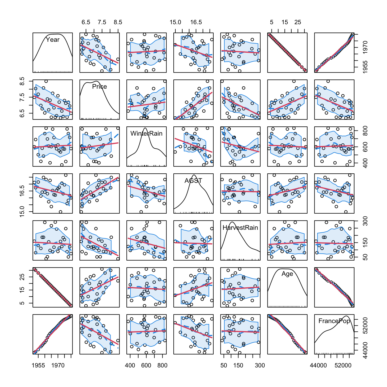

$Scatterplot matrix for the wine dataset. The diagonal plots show density estimators of the pdf of each variable (see Section 6.1.2). The $(i,j)$-th scatterplot shows the data of $X_i$ vs. $X_j,$ where the red line is the regression line of $X_i$ (response) on $X_j$ (predictor) and the blue curve represents a smoother that estimates nonparametrically the regression function of $X_i$ on $X_j$ (see Section 6.2). The dashed blue curves are the confidence intervals associated to the nonparametric smoother.$

Figure 2.5: Scatterplot matrix for the wine dataset. The diagonal plots show density estimators of the pdf of each variable (see Section 6.1.2). The $(i,j)$ -th scatterplot shows the data of $X_i$ vs. $X_j,$ where the red line is the regression line of $X_i$ (response) on $X_j$ (predictor) and the blue curve represents a smoother that estimates nonparametrically the regression function of $X_i$ on $X_j$ (see Section 6.2). The dashed blue curves are the confidence intervals associated to the nonparametric smoother.

As we can see, Year and FrancePop are very dependent, and Year and Age are perfectly dependent. This is so because Age = 1983 - Year. Therefore, we opt to remove the predictor Year and use it to set the case names, which can be helpful later for identifying outliers:

# Set row names to Year -- useful for outlier identification
row.names(wine) <- wine$Year
wine$Year <- NULL

Remember that the objective is to predict Price. Based on the above matrix scatterplot, the best we can predict Price by a simple linear regression seems to be with AGST or HarvestRain. Let’s see which one yields the higher $R^2,$ which, as we will see in Section 2.7.1, is an indicative of the performance of the linear model.

# Price ~ AGST
modAGST <- lm(Price ~ AGST, data = wine)

# Summary of the model
summary(modAGST)
## 
## Call:
## lm(formula = Price ~ AGST, data = wine)
## 
## Residuals:
##      Min       1Q   Median       3Q      Max 
## -0.78370 -0.23827 -0.03421  0.29973  0.90198 
## 
## Coefficients:
##             Estimate Std. Error t value Pr(>|t|)    
## (Intercept)  -3.5469     2.3641  -1.500 0.146052    
## AGST          0.6426     0.1434   4.483 0.000143 ***
## ---
## Signif. codes:  0 '***' 0.001 '**' 0.01 '*' 0.05 '.' 0.1 ' ' 1
## 
## Residual standard error: 0.4819 on 25 degrees of freedom
## Multiple R-squared:  0.4456, Adjusted R-squared:  0.4234 
## F-statistic: 20.09 on 1 and 25 DF,  p-value: 0.0001425

# The summary is also an object
sumModAGST <- summary(modAGST)
names(sumModAGST)
##  [1] "call"          "terms"         "residuals"     "coefficients"  "aliased"       "sigma"         "df"           
##  [8] "r.squared"     "adj.r.squared" "fstatistic"    "cov.unscaled"

# R^2
sumModAGST$r.squared
## [1] 0.4455894

Complete the analysis by computing the linear models Price ~ FrancePop, Price ~ Age, Price ~ WinterRain, and Price ~ HarvestRain. Name them as modFrancePop, modAge, modWinterRain, and modHarvestRain. Obtain their $R^2$ ’s and display them in a table like:

Predictor	$R^2$
`AGST`	$0.4456$
`HarvestRain`	$0.2572$
`FrancePop`	$0.2314$
`Age`	$0.2120$
`WinterRain`	$0.0181$

It seems that none of these simple linear models on their own are properly explaining Price. Intuitively, it would make sense to bind them together to achieve a better explanation of Price. Let’s see how to do that with a more advanced model.

2.2.3 Multiple linear model

The multiple linear model extends the simple linear model by describing the relation between several random variables $X_1,\ldots,X_p\;$ ¹⁹ and $Y.$ Therefore, as before, the multiple linear model is constructed by assuming that the linear relation

$\begin{align} Y = \beta_0 + \beta_1 X_1 + \cdots + \beta_p X_p + \varepsilon \tag{2.4} \end{align}$

holds between the predictors $X_1,\ldots,X_p$ and the response $Y.$ In (2.4), $\beta_0$ is the intercept and $\beta_1,\ldots,\beta_p$ are the slopes, respectively. The random variable $\varepsilon$ has mean zero and is independent from $X_1,\ldots,X_p.$ Another way of looking at (2.4) is

$\begin{align} \mathbb{E}[Y|X_1=x_1,\ldots,X_p=x_p]=\beta_0+\beta_1x_1+\cdots+\beta_px_p, \tag{2.5} \end{align}$

since $\mathbb{E}[\varepsilon|X_1=x_1,\ldots,X_p=x_p]=0.$

The LHS of (2.5) is the conditional expectation of $Y$ given $X_1,\ldots,$ $X_p.$ It represents how the mean of the random variable $Y$ is changing, now according to particular values of several predictors. With the RHS, what we are saying is that the mean of $Y$ is changing in a linear fashion with respect to the values of $X_1,\ldots,X_p.$ Hence the neat interpretation of the coefficients:

$\beta_0$ : is the mean of $Y$ when $X_1=\ldots=X_p=0.$
$\beta_j,$ $1\leq j\leq p$ : is the increment in the mean of $Y$ for an increment of one unit in $X_j=x_j,$ provided that the rest of predictors $X_1,\ldots,X_{j-1},X_{j+1},\ldots,X_p$ remain constant.

Figure 2.6 illustrates the geometrical interpretation of a multiple linear model: a hyperplane in $\mathbb{R}^{p+1}.$ If $p=1,$ the hyperplane is actually a line, the regression line for simple linear regression. If $p=2,$ then the regression plane can be visualized in a $3$ -dimensional plot.

The estimation of $\beta_0,\beta_1,\ldots,\beta_p$ is done as in simple linear regression by minimizing the RSS, which now accounts for the sum of squared distances of the data to the vertical projections on the hyperplane. Before doing so, we need to introduce some helpful matrix notation:

A sample of $(X_1,\ldots,X_p,Y)$ is denoted as $\{(X_{i1},\ldots,X_{ip},Y_i)\}_{i=1}^n,$ where $X_{ij}$ is the $i$ -th observation of the $j$ -th predictor $X_j.$ We denote with $\mathbf{X}_i:=(X_{i1},\ldots,X_{ip})$ to the $i$ -th observation of $(X_1,\ldots,X_p),$ so the sample simplifies to $\{(\mathbf{X}_{i},Y_i)\}_{i=1}^n.$
The design matrix contains all the information of the predictors plus a column of ones

$\begin{align*} \mathbf{X}:=\begin{pmatrix} 1 & X_{11} & \cdots & X_{1p}\\ \vdots & \vdots & \ddots & \vdots\\ 1 & X_{n1} & \cdots & X_{np} \end{pmatrix}_{n\times(p+1)}. \end{align*}$

The vector of responses $\mathbf{Y},$ the vector of coefficients $\boldsymbol{\beta},$ and the vector of errors are, respectively,

$\begin{align*} \mathbf{Y}:=\begin{pmatrix} Y_1 \\ \vdots \\ Y_n \end{pmatrix}_{n\times 1},\quad\boldsymbol{\beta}:=\begin{pmatrix} \beta_0 \\ \beta_1 \\ \vdots \\ \beta_p \end{pmatrix}_{(p+1)\times 1}\text{, and } \boldsymbol{\varepsilon}:=\begin{pmatrix} \varepsilon_1 \\ \vdots \\ \varepsilon_n \end{pmatrix}_{n\times 1}. \end{align*}$

Thanks to the matrix notation, we can turn the sample version²⁰ of the multiple linear model, namely

$\begin{align*} Y_i=\beta_0 + \beta_1 X_{i1} + \cdots +\beta_p X_{ip} + \varepsilon_i,\quad i=1,\ldots,n, \end{align*}$

into something as compact as

$\begin{align*} \mathbf{Y}=\mathbf{X}\boldsymbol{\beta}+\boldsymbol{\varepsilon}. \end{align*}$

Figure 2.6: The least squares regression plane $y=\hat\beta_0+\hat\beta_1x_1+\hat\beta_2x_2$ and its dependence on the kind of squared distance considered. Application available here.

Recall that if $p=1$ we recover the simple linear model. In this case:

$\begin{align*} \mathbf{X}=\begin{pmatrix} 1 & X_{11}\\ \vdots & \vdots\\ 1 & X_{n1} \end{pmatrix}_{n\times2}\text{ and } \boldsymbol{\beta}=\begin{pmatrix} \beta_0 \\ \beta_1 \end{pmatrix}_{2\times 1}. \end{align*}$

With this notation, the RSS for the multiple linear regression is

$\begin{align} \text{RSS}(\boldsymbol{\beta}):=&\,\sum_{i=1}^n(Y_i-\beta_0-\beta_1X_{i1}-\cdots-\beta_pX_{ip})^2\nonumber\\ =&\,(\mathbf{Y}-\mathbf{X}\boldsymbol{\beta})'(\mathbf{Y}-\mathbf{X}\boldsymbol{\beta}).\tag{2.6} \end{align}$

The RSS aggregates the squared vertical distances from the data to a regression plane given by $\boldsymbol{\beta}.$ The least squares estimators are the minimizers of the RSS²¹:

$\begin{align*} \hat{\boldsymbol{\beta}}:=\arg\min_{\boldsymbol{\beta}\in\mathbb{R}^{p+1}} \text{RSS}(\boldsymbol{\beta}). \end{align*}$

Luckily, thanks to the matrix form of (2.6), it is possible²² to compute a closed-form expression for the least squares estimates:

$\begin{align} \hat{\boldsymbol{\beta}}=(\mathbf{X}'\mathbf{X})^{-1}\mathbf{X}'\mathbf{Y}.\tag{2.7} \end{align}$

There are some similarities between (2.7) and

{\hat{β}}_{1} = (s_{x}^{2})^{- 1}

$\hat\beta_1=(s_x^2)^{-1}$

s_{x y}

$s_{xy}$ from the simple linear model: both are related to the covariance between

X

$\mathbf{X}$ and

Y

$Y$ weighted by the variance of

X .

$\mathbf{X}.$

Let’s check that indeed the coefficients given by lm are the ones given by (2.7). For that purpose we consider the leastSquares3D data frame in the least-squares-3D.RData dataset. Among other variables, the data frame contains the response yLin and the predictors x1 and x2.

load(file = "least-squares-3D.RData")

Let’s compute the coefficients of the regression of yLin on the predictors x1 and x2, which is denoted by yLin ~ x1 + x2. Note the use of + for including all the predictors. This does not mean that they are all added and then the regression is done on the sum.²³ Instead, this syntax is designed to resemble the mathematical form of the multiple linear model.

# Output from lm
mod <- lm(yLin ~ x1 + x2, data = leastSquares3D)
mod$coefficients
## (Intercept)          x1          x2 
##  -0.5702694   0.4832624   0.3214894

# Matrix X
X <- cbind(1, leastSquares3D$x1, leastSquares3D$x2)

# Vector Y
Y <- leastSquares3D$yLin

# Coefficients
beta <- solve(t(X) %*% X) %*% t(X) %*% Y
# %*% multiplies matrices
# solve() computes the inverse of a matrix
# t() transposes a matrix
beta
##            [,1]
## [1,] -0.5702694
## [2,]  0.4832624
## [3,]  0.3214894

Compute $\hat{\boldsymbol{\beta}}$ for the regressions yLin ~ x1 + x2, yQua ~ x1 + x2, and yExp ~ x2 + x3 using:

Equation (2.7) and
the function lm.

Check that both are the same.

Once we have the least squares estimates $\hat{\boldsymbol{\beta}},$ we can define the next concepts:

The fitted values $\hat Y_1,\ldots,\hat Y_n,$ where

$\begin{align*} \hat Y_i:=\hat\beta_0+\hat\beta_1X_{i1}+\cdots+\hat\beta_pX_{ip},\quad i=1,\ldots,n. \end{align*}$

They are the vertical projections of $Y_1,\ldots,Y_n$ onto the fitted plane (see Figure 2.6). In a matrix form, inputting (2.6)

$\begin{align*} \hat{\mathbf{Y}}=\mathbf{X}\hat{\boldsymbol{\beta}}=\mathbf{X}(\mathbf{X}'\mathbf{X})^{-1}\mathbf{X}'\mathbf{Y}=\mathbf{H}\mathbf{Y}, \end{align*}$

where $\mathbf{H}:=\mathbf{X}(\mathbf{X}'\mathbf{X})^{-1}\mathbf{X}'$ is called the hat matrix because it “puts the hat into $\mathbf{Y}$ ”. What it does is to project $\mathbf{Y}$ into the regression plane (see Figure 2.6).
The residuals (or estimated errors) $\hat \varepsilon_1,\ldots,\hat \varepsilon_n,$ where

$\begin{align*} \hat\varepsilon_i:=Y_i-\hat Y_i,\quad i=1,\ldots,n. \end{align*}$

They are the vertical distances between actual data and fitted data.

These two objects are present in the output of lm:

# Fitted values
mod$fitted.values

# Residuals
mod$residuals

We conclude with an important insight on the relation of multiple and simple linear regressions that is illustrated in Figure 2.7. The data used in that figure is:

set.seed(212542)
n <- 100
x1 <- rnorm(n, sd = 2)
x2 <- rnorm(n, mean = x1, sd = 3)
y <- 1 + 2 * x1 - x2 + rnorm(n, sd = 1)
data <- data.frame(x1 = x1, x2 = x2, y = y)

Consider the multiple linear model $Y=\beta_0+\beta_1X_1+\beta_2X_2$ $+\varepsilon_1$ and its associated simple linear models $Y=\alpha_0+\alpha_1X_1+\varepsilon_2$ and $Y=\gamma_0+\gamma_1X_2+\varepsilon_3,$ where $\varepsilon_1,\varepsilon_2,\varepsilon_3$ are random errors. Assume that we have a sample $\{(X_{i1},X_{i2},Y_i)\}_{i=1}^n.$ Then, in general, $\hat\alpha_0\neq\hat\beta_0\neq\hat\gamma_0,$ $\hat\alpha_1\neq\hat\beta_1,$ and $\hat\gamma_1\neq\hat\beta_2.$ Even if $\alpha_0=\beta_0=\gamma_0,$ $\alpha_1=\beta_1,$ and $\gamma_1=\beta_2.$ That is, in general, the inclusion of a new predictor changes the coefficient estimates of the rest of predictors.

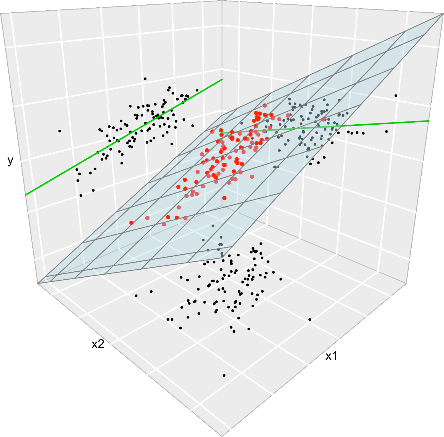
$The regression plane (blue) of $Y$ on $X_1$ and $X_2$ and its relation with the simple linear regressions (green lines) of $Y$ on $X_1$ and of $Y$ on $X_2.$ The red points represent the sample for $(X_1,X_2,Y)$ and the black points the sample projections for $(X_1,X_2)$ (bottom), $(X_1,Y)$ (left), and $(X_2,Y)$ (right). As it can be seen, the regression plane does not extend the simple linear regressions.$

Figure 2.7: The regression plane (blue) of $Y$ on $X_1$ and $X_2$ and its relation with the simple linear regressions (green lines) of $Y$ on $X_1$ and of $Y$ on $X_2.$ The red points represent the sample for $(X_1,X_2,Y)$ and the black points the sample projections for $(X_1,X_2)$ (bottom), $(X_1,Y)$ (left), and $(X_2,Y)$ (right). As it can be seen, the regression plane does not extend the simple linear regressions.

With the above data, check how the fitted coefficients change for y ~ x1, y ~ x2, and y ~ x1 + x2.

2.2.4 Case study application

A natural step now is to extend these simple regressions to increase both the $R^2$ and the prediction accuracy for Price by means of the multiple linear regression:

# Regression on all the predictors
modWine1 <- lm(Price ~ Age + AGST + FrancePop + HarvestRain + WinterRain,
               data = wine)

# A shortcut
modWine1 <- lm(Price ~ ., data = wine)
modWine1
## 
## Call:
## lm(formula = Price ~ ., data = wine)
## 
## Coefficients:
## (Intercept)   WinterRain         AGST  HarvestRain          Age    FrancePop  
##  -2.343e+00    1.153e-03    6.144e-01   -3.837e-03    1.377e-02   -2.213e-05

# Summary
summary(modWine1)
## 
## Call:
## lm(formula = Price ~ ., data = wine)
## 
## Residuals:
##      Min       1Q   Median       3Q      Max 
## -0.46541 -0.24133  0.00413  0.18974  0.52495 
## 
## Coefficients:
##               Estimate Std. Error t value Pr(>|t|)    
## (Intercept) -2.343e+00  7.697e+00  -0.304  0.76384    
## WinterRain   1.153e-03  4.991e-04   2.311  0.03109 *  
## AGST         6.144e-01  9.799e-02   6.270 3.22e-06 ***
## HarvestRain -3.837e-03  8.366e-04  -4.587  0.00016 ***
## Age          1.377e-02  5.821e-02   0.237  0.81531    
## FrancePop   -2.213e-05  1.268e-04  -0.175  0.86313    
## ---
## Signif. codes:  0 '***' 0.001 '**' 0.01 '*' 0.05 '.' 0.1 ' ' 1
## 
## Residual standard error: 0.293 on 21 degrees of freedom
## Multiple R-squared:  0.8278, Adjusted R-squared:  0.7868 
## F-statistic: 20.19 on 5 and 21 DF,  p-value: 2.232e-07

The fitted regression is Price $= -2.343 + 0.013\,\times$ Age $+ 0.614\,\times$ AGST $- 0.000\,\times$ FrancePop $- 0.003\,\times$ HarvestRain $+ 0.001\,\times$ WinterRain. Recall that the 'Multiple R-squared' has almost doubled with respect to the best simple linear regression! This tells us that combining several predictors may lead to important performance gains in the prediction of the response. However, note that the $R^2$ of the multiple linear model is not the sum of the $R^2$ ’s of the simple linear models. The performance gain of combining predictors is hard to anticipate from the single-predictor models and depends on the dependence among the predictors.

They are unique and always exist (except if $s_x=0,$ when all the data points are the same). They can be obtained by solving $\frac{\partial}{\partial \beta_0}\text{RSS}(\beta_0,\beta_1)=0$ and $\frac{\partial}{\partial \beta_1}\text{RSS}(\beta_0,\beta_1)=0.$ ↩︎
The sample standard deviation is $s_x=\sqrt{s_x^2}.$ ↩︎
Note that now $X_1$ represents the first predictor and not the first element of a sample of $X.$ ↩︎
Recall that (2.4) and (2.5) were referring to the relation of the random variable (or population) $Y$ with the random variables $X_1,\ldots,X_p.$ Those are population versions of the linear model and clearly generate the sample versions when they are replicated for each observation $(\mathbf{X}_{i},Y_i),$ $i=1,\ldots,n,$ of the random vector $(\mathbf{X},Y).$ ↩︎
It can be seen that they are unique and that they always exist, provided that $\mathrm{rank}(\mathbf{X}'\mathbf{X})=p+1.$ ↩︎
It follows from $\frac{\partial (\mathbf{A}\mathbf{x})}{\partial \mathbf{x}}=\mathbf{A}$ and $\frac{\partial (f(\mathbf{x})'g(\mathbf{x}))}{\partial \mathbf{x}}=f(\mathbf{x})'\frac{\partial g(\mathbf{x})}{\partial \mathbf{x}}+g(\mathbf{x})'\frac{\partial f(\mathbf{x})}{\partial \mathbf{x}}$ for two vector-valued functions $f,g:\mathbb{R}^p\rightarrow \mathbb{R}^m,$ where $\frac{\partial (f(\mathbf{x})'g(\mathbf{x}))}{\partial \mathbf{x}}$ is the gradient row vector of $f'g,$ and $\frac{\partial f(\mathbf{x})}{\partial \mathbf{x}}$ and $\frac{\partial g(\mathbf{x})}{\partial \mathbf{x}}$ are the Jacobian matrices of $f$ and $g,$ respectively.↩︎
If you wanted to do so, you will need to use the function I() for indicating that + is not including predictors in the model, but is acting as the algebraic sum operator.↩︎