5.8 Shrinkage
Enforcing sparsity in generalized linear models can be done as how it was done in linear models. Ridge regression and lasso can be generalized with glmnet with little differences in practice.
What we want is to bias the estimates of \(\boldsymbol{\beta}\) towards being non-null only in the most important relations between the response and predictors. To achieve that, we add a penalization term to the maximum likelihood estimation of \(\boldsymbol{\beta}\):185
\[\begin{align} -\ell(\boldsymbol{\beta})+\lambda\sum_{j=1}^p (\alpha|\beta_j|+(1-\alpha)|\beta_j|^2).\tag{5.38} \end{align}\]
As in Section 4.1, ridge regression corresponds to \(\alpha=0\) (quadratic penalty) and lasso to \(\alpha=1\) (absolute value penalty). Obviously, if \(\lambda=0,\) we are back to the generalized linear models theory. The optimization of (5.38) gives
\[\begin{align} \hat{\boldsymbol{\beta}}_{\lambda,\alpha}:=\arg\min_{\boldsymbol{\beta}\in\mathbb{R}^{p+1}}\left\{ -\ell(\boldsymbol{\beta})+\lambda\sum_{j=1}^p (\alpha|\beta_j|+(1-\alpha)|\beta_j|^2)\right\}.\tag{5.39} \end{align}\]
Note that the sparsity is enforced in the slopes, not in the intercept, and that the link function \(g\) is not affecting the penalization term. As in linear models, the predictors need to be standardized if they have a different nature.
We illustrate the shrinkage in generalized linear models with the ISLR::Hitters dataset, where now the objective will be to predict NewLeague, a factor with levels A (standing for American League) and N (standing for National League). The variable indicates the player’s league at the end of 1986. The predictors employed are his statistics during 1986, and the objective is to see whether there is some distinctive pattern between the players in both leagues.
# Load data
data(Hitters, package = "ISLR")

# Include only predictors related with 1986 season and discard NA's
Hitters <- subset(Hitters, select = c(League, AtBat, Hits, HmRun, Runs, RBI,
                                      Walks, Division, PutOuts, Assists,
                                      Errors))
Hitters <- na.omit(Hitters)

# Response and predictors
y <- Hitters$League
x <- model.matrix(League ~ ., data = Hitters)[, -1]
After preparing the data, we perform the regressions.
# Ridge and lasso regressions
library(glmnet)
ridgeMod <- glmnet(x = x, y = y, alpha = 0, family = "binomial")
lassoMod <- glmnet(x = x, y = y, alpha = 1, family = "binomial")

# Solution paths versus lambda
plot(ridgeMod, label = TRUE, xvar = "lambda")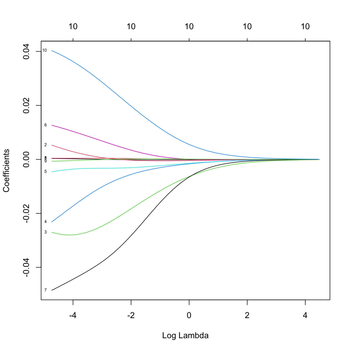

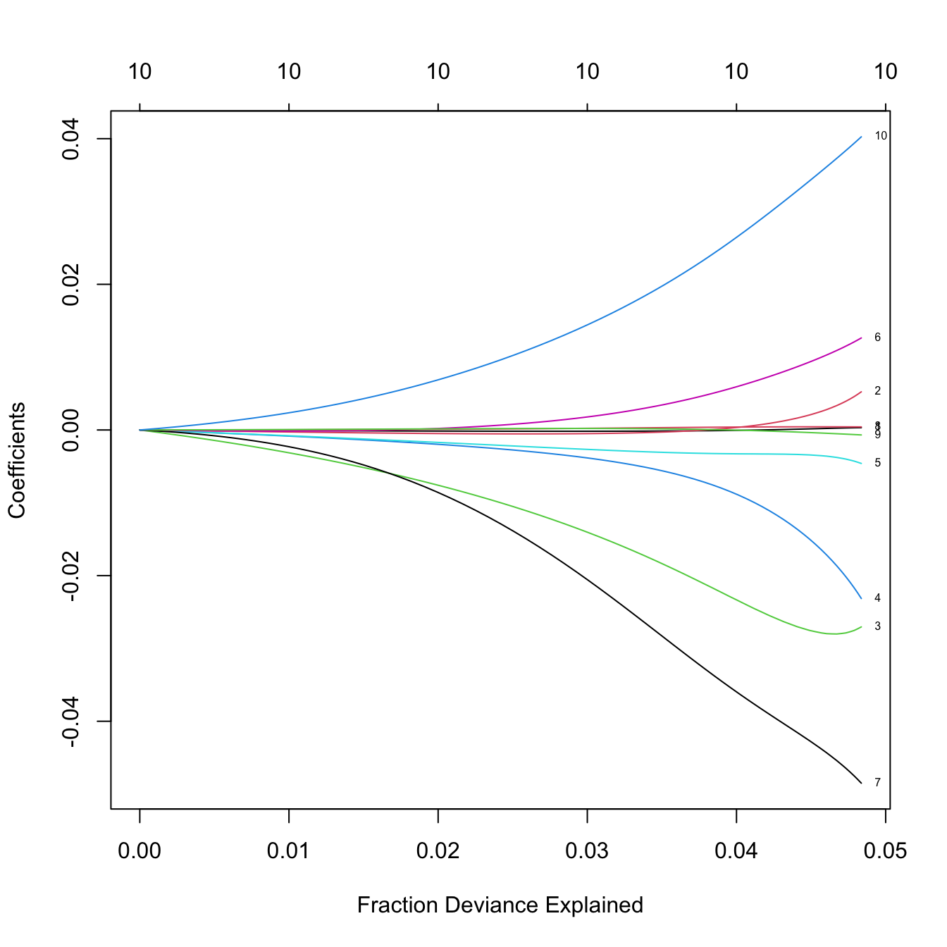

# The percentage of deviance explained only goes up to 0.05. There are no
# clear patterns indicating player differences between both leagues

# Let's select the predictors to be included with a 10-fold cross-validation
set.seed(12345)
kcvLasso <- cv.glmnet(x = x, y = y, alpha = 1, nfolds = 10, family = "binomial")
plot(kcvLasso)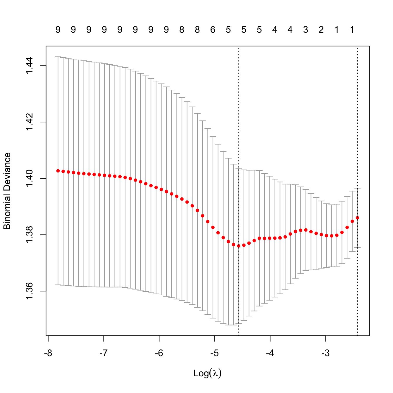
# The lambda that minimizes the CV error and "one standard error rule"'s lambda
kcvLasso$lambda.min
## [1] 0.01039048
kcvLasso$lambda.1se
## [1] 0.08829343

# Leave-one-out cross-validation -- similar result
ncvLasso <- cv.glmnet(x = x, y = y, alpha = 1, nfolds = nrow(Hitters),
                      family = "binomial")
plot(ncvLasso)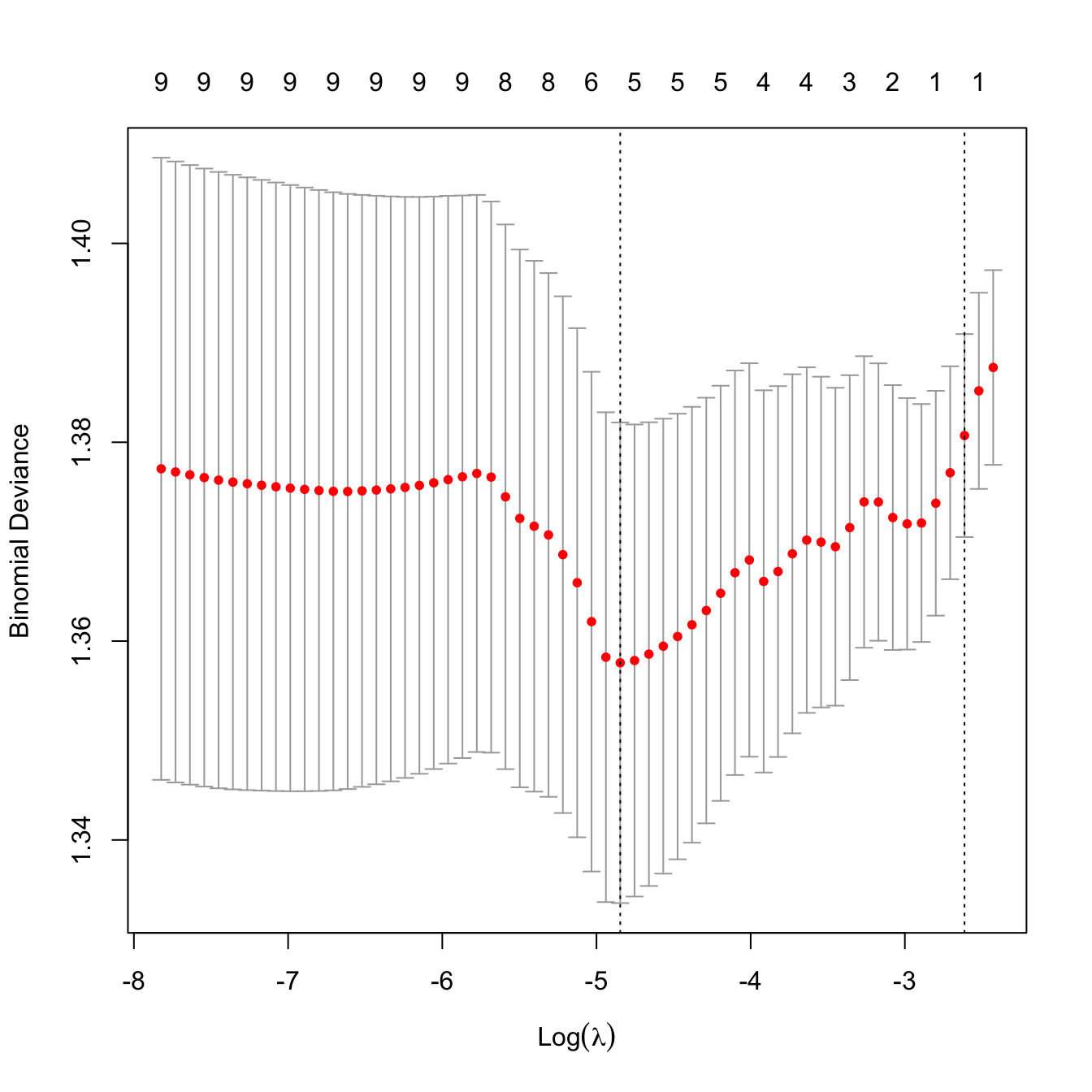
ncvLasso$lambda.min
## [1] 0.007860015
ncvLasso$lambda.1se
## [1] 0.07330276

# Model selected
predict(ncvLasso, type = "coefficients", s = ncvLasso$lambda.1se)
## 11 x 1 sparse Matrix of class "dgCMatrix"
##                       s1
## (Intercept) -0.099447861
## AtBat        .
## Hits         .
## HmRun       -0.006971231
## Runs         .
## RBI          .
## Walks        .
## DivisionW    .
## PutOuts      .
## Assists      .
## Errors       .
HmRun is selected by leave-one-out cross-validation as the unique predictor to be included in the lasso regression. We know that the model is not good due to the percentage of deviance explained. However, we still want to know whether HmRun has any significance at all. When addressing this, we have to take into account Appendix A.5 to avoid spurious findings.
# Analyze the selected model
fit <- glm(League ~ HmRun, data = Hitters, family = "binomial")
summary(fit)
##
## Call:
## glm(formula = League ~ HmRun, family = "binomial", data = Hitters)
##
## Deviance Residuals:
##     Min       1Q   Median       3Q      Max
## -1.2976  -1.1320  -0.8106   1.1686   1.6440
##
## Coefficients:
##             Estimate Std. Error z value Pr(>|z|)
## (Intercept)  0.27826    0.18086   1.539  0.12392
## HmRun       -0.04290    0.01371  -3.130  0.00175 **
## ---
## Signif. codes:  0 '***' 0.001 '**' 0.01 '*' 0.05 '.' 0.1 ' ' 1
##
## (Dispersion parameter for binomial family taken to be 1)
##
##     Null deviance: 443.95  on 321  degrees of freedom
## Residual deviance: 433.57  on 320  degrees of freedom
## AIC: 437.57
##
## Number of Fisher Scoring iterations: 4
# HmRun is significant -- but it may be spurious due to the model selection
# procedure (see Appendix A.5)

# Let's split the dataset in two, do model-selection in one part and then
# inference on the selected model in the other, to have an idea of the real
# significance of HmRun
set.seed(12345678)
train <- sample(c(FALSE, TRUE), size = nrow(Hitters), replace = TRUE)

# Model selection in training part
ncvLasso <- cv.glmnet(x = x[train, ], y = y[train], alpha = 1,
                      nfolds = sum(train), family = "binomial")
predict(ncvLasso, type = "coefficients", s = ncvLasso$lambda.1se)
## 11 x 1 sparse Matrix of class "dgCMatrix"
##                      s1
## (Intercept)  0.27240020
## AtBat        .
## Hits         .
## HmRun       -0.01255322
## Runs         .
## RBI          .
## Walks        .
## DivisionW    .
## PutOuts      .
## Assists      .
## Errors       .

# Inference in testing part
summary(glm(League ~ HmRun, data = Hitters[!train, ], family = "binomial"))
##
## Call:
## glm(formula = League ~ HmRun, family = "binomial", data = Hitters[!train,
##     ])
##
## Deviance Residuals:
##     Min       1Q   Median       3Q      Max
## -1.1170  -1.0177  -0.8517   1.3173   1.6896
##
## Coefficients:
##             Estimate Std. Error z value Pr(>|z|)
## (Intercept) -0.14389    0.25754  -0.559   0.5764
## HmRun       -0.03255    0.01955  -1.665   0.0958 .
## ---
## Signif. codes:  0 '***' 0.001 '**' 0.01 '*' 0.05 '.' 0.1 ' ' 1
##
## (Dispersion parameter for binomial family taken to be 1)
##
##     Null deviance: 216.54  on 162  degrees of freedom
## Residual deviance: 213.64  on 161  degrees of freedom
## AIC: 217.64
##
## Number of Fisher Scoring iterations: 4
# HmRun is now not significant...
# We can repeat the analysis for different partitions of the data and we will
# obtain weak significances. Therefore, we can conclude that this is an spurious
# finding and that HmRun is not significant as a single predictor

# Prediction (obviously not trustable, but for illustration)
pred <- predict(ncvLasso, newx = x[!train, ], type = "response",
                s = ncvLasso$lambda.1se)

# Hit matrix and hit ratio
H <- table(pred > 0.5, y[!train] == "A") # ("A" was the reference level)
H
##
##         FALSE TRUE
##   FALSE     5   18
##   TRUE     57   83
sum(diag(H)) / sum(H) # Almost like tossing a coin!
## [1] 0.5398773
From the above analysis, we can conclude that there are no significative differences between the players of both leagues in terms of the variables analyzed.
Perform an adequate statistical analysis based on shrinkage of a generalized linear model to reply the following questions:
- What (if any) are the leading factors among the features of a player in season 1986 in order to be in the top \(10\%\) of most paid players in season 1987?
- What (if any) are the player features in season 1986 influencing the number of home runs in the same season? And during his career?
We are now minimizing \(-\ell(\boldsymbol{\beta}),\) the negative log-likelihood.↩︎