5.5 Deviance

The deviance is a key concept in generalized linear models. Intuitively, it measures the deviance of the fitted generalized linear model with respect to a perfect model for the sample $\{(\mathbf{x}_i,Y_i)\}_{i=1}^n.$ This perfect model, known as the saturated model, is the model that perfectly fits the data, in the sense that the fitted responses ($\hat Y_i$) equal the observed responses ($Y_i$). For example, in logistic regression this would be the model such that

$$\begin{align*} \hat{\mathbb{P}}[Y=1|X_1=X_{i1},\ldots,X_p=X_{ip}]=Y_i,\quad i=1,\ldots,n. \end{align*}$$

Figure 5.9 shows a¹⁷⁴ saturated model and a fitted logistic model.

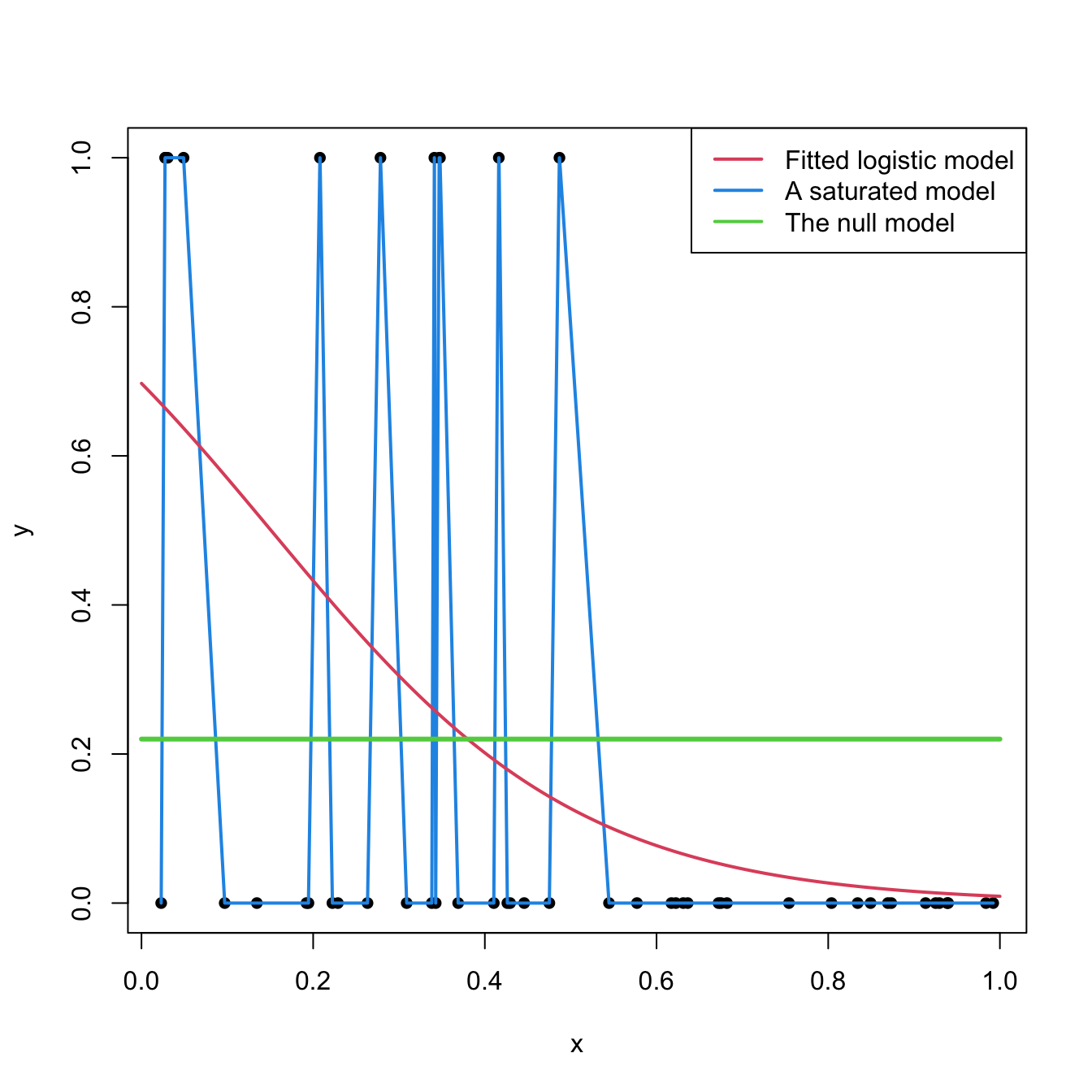
Figure 5.9: Fitted logistic regression versus a saturated model and the null model.

Formally, the deviance is defined through the difference of the log-likelihoods between the fitted model, $\ell(\hat{\boldsymbol{\beta}}),$ and the saturated model, $\ell_s.$ Computing $\ell_s$ amounts to substitute $\mu_i$ by $Y_i$ in (5.20). If the canonical link function is used, this corresponds to setting $\theta_i=g(Y_i)$ (recall (5.12)). The deviance is then defined as:

$$\begin{align*} D:=-2\left[\ell(\hat{\boldsymbol{\beta}})-\ell_s\right]\phi. \end{align*}$$

The log-likelihood $\ell(\hat{\boldsymbol{\beta}})$ is always smaller than $\ell_s$ (the saturated model is more likely given the sample, since it is the sample itself). As a consequence, the deviance is always larger or equal than zero, being zero only if the fit of the model is perfect.

If the canonical link function is employed, the deviance can be expressed as

$$\begin{align} D&=-\frac{2}{a(\phi)}\sum_{i=1}^n\left(Y_i\hat\theta_i-b(\hat\theta_i)-Y_ig(Y_i)+b(g(Y_i))\right)\phi\nonumber\\ &=\frac{2\phi}{a(\phi)}\sum_{i=1}^n\left(Y_i(g(Y_i)-\hat\theta_i)-b(g(Y_i))+b(\hat\theta_i)\right).\tag{5.30} \end{align}$$

In most of the cases, $a(\phi)\propto\phi,$ so the deviance does not depend on $\phi$. Expression (5.30) is interesting, since it delivers the following key insight:

The deviance generalizes the Residual Sum of Squares (RSS) of the linear model. The generalization is driven by the likelihood and its equivalence with the RSS in the linear model.

To see this insight, let’s consider the linear model in (5.30) by setting $\phi=\sigma^2,$ $a(\phi)=\phi,$ $b(\theta)=\frac{\theta^2}{2},$ $c(y,\phi)=-\frac{1}{2}\{\frac{y^2}{\phi}+\log(2\pi\phi)\},$ and $\theta=\mu=\eta.$¹⁷⁵ Then:

$$\begin{align} D&=\frac{2\sigma^2}{\sigma^2}\sum_{i=1}^n\left(Y_i(Y_i-\hat{\eta}_i)-\frac{Y_i^2}{2}+\frac{\hat{\eta}_i^2}{2}\right)\nonumber\\ &=\sum_{i=1}^n\left(2Y_i^2-2Y_i\hat{\eta}_i-Y_i^2+\hat{\eta}_i^2\right)\nonumber\\ &=\sum_{i=1}^n\left(Y_i-\hat{\eta}_i\right)^2\nonumber\\ &=\mathrm{RSS}(\hat{\boldsymbol{\beta}}),\tag{5.31} \end{align}$$

since $\hat{\eta}_i=\hat\beta_0+\hat\beta_1x_{i1}+\cdots+\hat\beta_px_{ip}.$ Remember that $\mathrm{RSS}(\hat{\boldsymbol{\beta}})$ is just another name for the SSE.

A benchmark for evaluating the scale of the deviance is the null deviance,

$$\begin{align*} D_0:=-2\left[\ell(\hat{\beta}_0)-\ell_s\right]\phi, \end{align*}$$

which is the deviance of the model without predictors, the one featuring only an intercept, to the perfect model. In logistic regression, this model is

$$\begin{align*} Y|(X_1=x_1,\ldots,X_p=x_p)\sim \mathrm{Ber}(\mathrm{logistic}(\beta_0)) \end{align*}$$

and, in this case, $\hat\beta_0=\mathrm{logit}(\frac{m}{n})=\log\left(\frac{\frac{m}{n}}{1-\frac{m}{n}}\right)$ where $m$ is the number of $1$’s in $Y_1,\ldots,Y_n$ (see Figure 5.9).

Using again (5.30), we can see that the null deviance is a generalization of the total sum of squares of the linear model (see Section 2.6):

$$\begin{align*} D_0=\sum_{i=1}^n\left(Y_i-\hat{\eta}_i\right)^2=\sum_{i=1}^n\left(Y_i-\hat\beta_0\right)^2=\mathrm{SST}, \end{align*}$$

since $\hat\beta_0=\bar Y$ because there are no predictors.

Figure 5.10: Pictorial representation of the deviance ($D$) and the null deviance ($D_0$).

Using the deviance and the null deviance, we can compare how much the model has improved by adding the predictors $X_1,\ldots,X_p$ and quantify the percentage of deviance explained. This can be done by means of the $R^2$ statistic, which is a generalization of the determination coefficient for linear regression:

$$\begin{align*} R^2:=1-\frac{D}{D_0}\stackrel{\substack{\mathrm{linear}\\ \mathrm{model}\\{}}}{=}1-\frac{\mathrm{SSE}}{\mathrm{SST}}. \end{align*}$$

The $R^2$ for generalized linear models is a measure that shares the same philosophy with the determination coefficient in linear regression: it is a proportion of how good the model fit is. If perfect, $D=0$ and $R^2=1.$ If the predictors are not model-related with $Y,$ then $D=D_0$ and $R^2=0.$

However, this $R^2$ has a different interpretation than in linear regression. In particular:

• Is not the percentage of variance explained by the model, but rather a ratio indicating how close is the fit to being perfect or the worst.
• It is not related to any correlation coefficient.

The deviance is returned by summary. It is important to recall that R refers to the deviance as the 'Residual deviance' and the null deviance is referred to as 'Null deviance'.

# Summary of model
nasa <- glm(fail.field ~ temp, family = "binomial", data = challenger)
summaryLog <- summary(nasa)
summaryLog
## 
## Call:
## glm(formula = fail.field ~ temp, family = "binomial", data = challenger)
## 
## Deviance Residuals: 
##     Min       1Q   Median       3Q      Max  
## -1.0566  -0.7575  -0.3818   0.4571   2.2195  
## 
## Coefficients:
##             Estimate Std. Error z value Pr(>|z|)  
## (Intercept)   7.5837     3.9146   1.937   0.0527 .
## temp         -0.4166     0.1940  -2.147   0.0318 *
## ---
## Signif. codes:  0 '***' 0.001 '**' 0.01 '*' 0.05 '.' 0.1 ' ' 1
## 
## (Dispersion parameter for binomial family taken to be 1)
## 
##     Null deviance: 28.267  on 22  degrees of freedom
## Residual deviance: 20.335  on 21  degrees of freedom
## AIC: 24.335
## 
## Number of Fisher Scoring iterations: 5
# 'Residual deviance' is the deviance; 'Null deviance' is the null deviance

# Null model (only intercept)
null <- glm(fail.field ~ 1, family = "binomial", data = challenger)
summaryNull <- summary(null)
summaryNull
## 
## Call:
## glm(formula = fail.field ~ 1, family = "binomial", data = challenger)
## 
## Deviance Residuals: 
##    Min      1Q  Median      3Q     Max  
## -0.852  -0.852  -0.852   1.542   1.542  
## 
## Coefficients:
##             Estimate Std. Error z value Pr(>|z|)  
## (Intercept)  -0.8267     0.4532  -1.824   0.0681 .
## ---
## Signif. codes:  0 '***' 0.001 '**' 0.01 '*' 0.05 '.' 0.1 ' ' 1
## 
## (Dispersion parameter for binomial family taken to be 1)
## 
##     Null deviance: 28.267  on 22  degrees of freedom
## Residual deviance: 28.267  on 22  degrees of freedom
## AIC: 30.267
## 
## Number of Fisher Scoring iterations: 4

# Compute the R^2 with a function -- useful for repetitive computations
r2glm <- function(model) {

  summaryLog <- summary(model)
  1 - summaryLog$deviance / summaryLog$null.deviance

}

# R^2
r2glm(nasa)
## [1] 0.280619
r2glm(null)
## [1] -4.440892e-16

A quantity related with the deviance is the scaled deviance:

$$\begin{align*} D^*:=\frac{D}{\phi}=-2\left[\ell(\hat{\boldsymbol{\beta}})-\ell_s\right]. \end{align*}$$

If $\phi=1,$ such as in the binomial or Poisson regression models, then both the deviance and the scaled deviance agree. The scaled deviance has asymptotic distribution

$$\begin{align} D^*\stackrel{a}{\sim}\chi^2_{n-p-1},\tag{5.32} \end{align}$$

where $\chi^2_{k}$ is the Chi-squared distribution with $k$ degrees of freedom. In the case of the linear model, $D^*=\frac{1}{\sigma^2}\mathrm{RSS}$ is exactly distributed as a $\chi^2_{n-p-1}.$

The result (5.32) provides a way of estimating $\phi$ when it is unknown: match $D^*$ with the expectation $\mathbb{E}\left[\chi^2_{n-p-1}\right]=n-p-1.$ This provides

$$\begin{align*} \hat\phi_D:=\frac{-2(\ell(\hat{\boldsymbol{\beta}})-\ell_s)}{n-p-1}, \end{align*}$$

which, as expected, in the case of the linear model is equivalent to $\hat\sigma^2$ as given in (2.15). More importantly, the scaled deviance can be used for performing hypotheses tests on sets of coefficients of a generalized linear model.

Assume we have one model, say $M_2,$ with $p_2$ predictors and another model, say $M_1$, with $p_1<p_2$ predictors that are contained in the set of predictors of the M2. In other words, assume $M_1$ is nested within $M_2.$ Then we can test the null hypothesis that the extra coefficients of $M_2$ are simultaneously zero. For example, if $M_1$ has the coefficients $\{\beta_0,\beta_1,\ldots,\beta_{p_1}\}$ and M2 has coefficients $\{\beta_0,\beta_1,\ldots,\beta_{p_1},\beta_{p_1+1},\ldots,\beta_{p_2}\},$ we can test

$$\begin{align*} H_0:\beta_{p_1+1}=\ldots=\beta_{p_2}=0\quad\text{vs.}\quad H_1:\beta_j\neq 0\text{ for any }p_1<j\leq p_2. \end{align*}$$

This can be done by means of the statistic¹⁷⁶

$$\begin{align} D^*_{p_1}-D^*_{p_2}\stackrel{a,\,H_0}{\sim}\chi^2_{p_2-p_1}.\tag{5.33} \end{align}$$

If $H_0$ is true,¹⁷⁷ then $D_{p_1}^*-D^*_{p_2}$ is expected to be small, thus we will reject $H_0$ if the value of the statistic is above the $\alpha$-upper quantile of the $\chi^2_{p_2-p_1}$, denoted as $\chi^2_{\alpha;p_2-p_1}.$

$D^*$ apparently removes the effects of $\phi,$ but it is still dependent on $\phi,$ since this is hidden in the likelihood (see (5.30)). Therefore, $D^*$ cannot be computed unless $\phi$ is known, which forbids using (5.33). Hopefully, this dependence is removed by employing (5.32) and (5.33) and assuming that they are asymptotically independent. This gives the $F$-test for $H_0$:

$$\begin{align*} F=\frac{(D^*_{p_1}-D^*_{p_2})/(p_2-p_1)}{D^*_{p_2}/(n-p_2-1)}=\frac{(D_{p_1}-D_{p_2})/(p_2-p_1)}{D_{p_2}/(n-p_2-1)}\stackrel{a,\,H_0}{\sim} F_{p_2-p_1,n-p_2-1}. \end{align*}$$

Note that $F$ is perfectly computable, since $\phi$ cancels due to the quotient (and because we assume that $a(\phi)\propto\phi$).

Note also that this is an extension of the $F$-test seen in Section 2.6: take $p_1=0$ and $p_2=p$ and then one tests the significance of all the predictors included in the model (both models contain intercept).

The computation of deviances and associated tests is done through anova, which implements the Analysis of Deviance. This is illustrated in the following code, which coincidentally also illustrates the inclusion of nonlinear transformations on the predictors.

# Polynomial predictors
nasa0 <- glm(fail.field ~ 1, family = "binomial", data = challenger)
nasa1 <- glm(fail.field ~ temp, family = "binomial", data = challenger)
nasa2 <- glm(fail.field ~ poly(temp, degree = 2), family = "binomial",
             data = challenger)
nasa3 <- glm(fail.field ~ poly(temp, degree = 3), family = "binomial",
             data = challenger)

# Plot fits
temp <- seq(-1, 35, l = 200)
tt <- data.frame(temp = temp)
plot(fail.field ~ temp, data = challenger, pch = 16, xlim = c(-1, 30),
     xlab = "Temperature", ylab = "Incident probability")
lines(temp, predict(nasa0, newdata = tt, type = "response"), col = 1)
lines(temp, predict(nasa1, newdata = tt, type = "response"), col = 2)
lines(temp, predict(nasa2, newdata = tt, type = "response"), col = 3)
lines(temp, predict(nasa3, newdata = tt, type = "response"), col = 4)
legend("bottomleft", legend = c("Null model", "Linear", "Quadratic", "Cubic"),
       lwd = 2, col = 1:4)

# R^2's
r2glm(nasa0)
## [1] -4.440892e-16
r2glm(nasa1)
## [1] 0.280619
r2glm(nasa2)
## [1] 0.3138925
r2glm(nasa3)
## [1] 0.4831863

# Chisq and F tests -- same results since phi is known
anova(nasa1, test = "Chisq")
## Analysis of Deviance Table
## 
## Model: binomial, link: logit
## 
## Response: fail.field
## 
## Terms added sequentially (first to last)
## 
## 
##      Df Deviance Resid. Df Resid. Dev Pr(>Chi)   
## NULL                    22     28.267            
## temp  1   7.9323        21     20.335 0.004856 **
## ---
## Signif. codes:  0 '***' 0.001 '**' 0.01 '*' 0.05 '.' 0.1 ' ' 1
anova(nasa1, test = "F")
## Analysis of Deviance Table
## 
## Model: binomial, link: logit
## 
## Response: fail.field
## 
## Terms added sequentially (first to last)
## 
## 
##      Df Deviance Resid. Df Resid. Dev      F   Pr(>F)   
## NULL                    22     28.267                   
## temp  1   7.9323        21     20.335 7.9323 0.004856 **
## ---
## Signif. codes:  0 '***' 0.001 '**' 0.01 '*' 0.05 '.' 0.1 ' ' 1

# Incremental comparisons of nested models
anova(nasa1, nasa2, nasa3, test = "Chisq")
## Analysis of Deviance Table
## 
## Model 1: fail.field ~ temp
## Model 2: fail.field ~ poly(temp, degree = 2)
## Model 3: fail.field ~ poly(temp, degree = 3)
##   Resid. Df Resid. Dev Df Deviance Pr(>Chi)  
## 1        21     20.335                       
## 2        20     19.394  1   0.9405   0.3321  
## 3        19     14.609  1   4.7855   0.0287 *
## ---
## Signif. codes:  0 '***' 0.001 '**' 0.01 '*' 0.05 '.' 0.1 ' ' 1
# Quadratic effects are not significative

# Cubic vs. linear
anova(nasa1, nasa3, test = "Chisq")
## Analysis of Deviance Table
## 
## Model 1: fail.field ~ temp
## Model 2: fail.field ~ poly(temp, degree = 3)
##   Resid. Df Resid. Dev Df Deviance Pr(>Chi)  
## 1        21     20.335                       
## 2        19     14.609  2    5.726   0.0571 .
## ---
## Signif. codes:  0 '***' 0.001 '**' 0.01 '*' 0.05 '.' 0.1 ' ' 1

# Example in Poisson regression
species1 <- glm(Species ~ ., data = species, family = poisson)
species2 <- glm(Species ~ Biomass * pH, data = species, family = poisson)

# Comparison
anova(species1, species2, test = "Chisq")
## Analysis of Deviance Table
## 
## Model 1: Species ~ pH + Biomass
## Model 2: Species ~ Biomass * pH
##   Resid. Df Resid. Dev Df Deviance  Pr(>Chi)    
## 1        86     99.242                          
## 2        84     83.201  2    16.04 0.0003288 ***
## ---
## Signif. codes:  0 '***' 0.001 '**' 0.01 '*' 0.05 '.' 0.1 ' ' 1
r2glm(species1)
## [1] 0.7806071
r2glm(species2)
## [1] 0.8160674

---

174. Several are possible depending on the interpolation between points.↩︎

175. The canonical link function $g$ is the identity, check (5.12) and (5.13).↩︎

176. Note that $D_{p_1}^*>D^*_{p_2}$ because $\ell(\hat{\boldsymbol{\beta}}_{p_1})<\ell(\hat{\boldsymbol{\beta}}_{p_2}).$↩︎

177. In other words, $M_2$ does not add significant predictors when compared with the submodel $M_1.$↩︎