B.3 Introduction to R
This section provides a collection of self-explainable code snippets for the programming language R (R Core Team 2020). These snippets are not meant to provide an exhaustive introduction to R but just to illustrate the very basic functions and methods.
In the following, # denotes comments to the code and ## outputs of the code.
Simple computations
# The console can act as a simple calculator
1.0 + 1.1
2 * 2
3/2
2^3
1/0
0/0

# Use ";" for performing several operations in the same line
(1 + 3) * 2 - 1; 3 + 2

# Elemental mathematical functions
sqrt(2); 2^0.5
exp(1)
log(10) # Natural logarithm
log10(10); log2(10) # Logs in base 10 and 2
sin(pi); cos(0); asin(0)
tan(pi/3)
sqrt(-1)

# Remember to close the parenthesis -- errors below
1 +
(1 + 3
## Error in parse(text = input): <text>:24:0: unexpected end of input
## 22: 1 +
## 23: (1 + 3
##    ^
Compute:
- \(\frac{e^{2}+\sin(2)}{\cos^{-1}\left(\tfrac{1}{2}\right)+2}.\) Answer:
2.723274. - \(\sqrt{3^{2.5}+\log(10)}.\) Answer:
4.22978. - \((2^{0.93}-\log_2(3 + \sqrt{2+\sin(1)}))10^{\tan(1/3))}\sqrt{3^{2.5}+\log(10)}.\) Answer:
-3.032108.
Variables and assignment
# Any operation that you perform in R can be stored in a variable
# (or object) with the assignment operator "<-"
x <- 1

# To see the value of a variable, simply type it
x
## [1] 1

# A variable can be overwritten
x <- 1 + 1

# Now the value of x is 2 and not 1, as before
x
## [1] 2

# Capitalization matters
X <- 3
x; X
## [1] 2
## [1] 3

# See what are the variables in the workspace
ls()
## [1] "x" "X"

# Remove variables
rm(X)
X
## Error in eval(expr, envir, enclos): object 'X' not found
Do the following:
- Store \(-123\) in the variable
y. - Store the log of the square of
yinz. - Store \(\frac{y-z}{y+z^2}\) in
yand removez. - Output the value of
y. Answer:4.366734.
Vectors
# We combine numbers with the function "c"
c(1, 3)
## [1] 1 3
c(1.5, 0, 5, -3.4)
## [1]  1.5  0.0  5.0 -3.4

# A handy way of creating integer sequences is the operator ":"
1:5
## [1] 1 2 3 4 5

# Storing some vectors
myData <- c(1, 2)
myData2 <- c(-4.12, 0, 1.1, 1, 3, 4)
myData
## [1] 1 2
myData2
## [1] -4.12  0.00  1.10  1.00  3.00  4.00

# Entrywise operations
myData + 1
## [1] 2 3
myData^2
## [1] 1 4

# If you want to access a position of a vector, use [position]
myData[1]
## [1] 1
myData2[6]
## [1] 4

# You can also change elements
myData[1] <- 0
myData
## [1] 0 2

# Think on what you want to access...
myData2[7]
## [1] NA
myData2[0]
## numeric(0)

# If you want to access all the elements except a position,
# use [-position]
myData2[-1]
## [1] 0.0 1.1 1.0 3.0 4.0
myData2[-2]
## [1] -4.12  1.10  1.00  3.00  4.00

# Also with vectors as indexes
myData2[1:2]
## [1] -4.12  0.00
myData2[myData]
## [1] 0

# And also
myData2[-c(1, 2)]
## [1] 1.1 1.0 3.0 4.0

# But do not mix positive and negative indexes!
myData2[c(-1, 2)]
## Error in myData2[c(-1, 2)]: only 0's may be mixed with negative subscripts

# Remove the first element
myData2 <- myData2[-1]
Do the following:
- Create the vector \(x=(1, 7, 3, 4).\)
- Create the vector \(y=(100, 99, 98, ..., 2, 1).\)
- Create the vector \(z=(4, 8, 16, 32, 96).\)
- Compute \(x_2+y_4\) and \(\cos(x_3) + \sin(x_2) e^{-y_2}.\) Answers:
104and-0.9899925. - Set \(x_{2}=0\) and \(y_{2}=-1.\) Recompute the previous expressions. Answers:
97and2.785875. - Index \(y\) by \(x+1\) and store it as
z. What is the output? Answer:zisc(-1, 100, 97, 96).
Some functions
# Functions take arguments between parenthesis and transform them
# into an output
sum(myData)
## [1] 2
prod(myData)
## [1] 0

# Summary of an object
summary(myData)
##    Min. 1st Qu.  Median    Mean 3rd Qu.    Max.
##     0.0     0.5     1.0     1.0     1.5     2.0

# Length of the vector
length(myData)
## [1] 2

# Mean, standard deviation, variance, covariance, correlation
mean(myData)
## [1] 1
var(myData)
## [1] 2
cov(myData, myData^2)
## [1] 4
cor(myData, myData * 2)
## [1] 1
quantile(myData)
##   0%  25%  50%  75% 100%
##  0.0  0.5  1.0  1.5  2.0

# Maximum and minimum of vectors
min(myData)
## [1] 0
which.min(myData)
## [1] 1

# Usually the functions have several arguments, which are set
# by "argument = value" In the next case, the second argument is
# a logical flag to indicate the kind of sorting
sort(myData) # If nothing is specified, decreasing = FALSE is
## [1] 0 2
# assumed
sort(myData, decreasing = TRUE)
## [1] 2 0

# Do not know what are the arguments of a function? Use args
# and help!
args(mean)
## function (x, ...)
## NULL
?mean
Do the following:
- Compute the mean, median and variance of \(y.\) Answers:
49.5,49.5,843.6869. - Do the same for \(y+1.\) What are the differences?
- What is the maximum of \(y\)? Where is it placed?
- Sort \(y\) increasingly and obtain the 5th and 76th positions. Answer:
c(4, 75). - Compute the covariance between \(y\) and \(y.\) Compute the variance of \(y.\) Why do you get the same result?
Matrices, data frames, and lists
# A matrix is an array of vectors
A <- matrix(1:4, nrow = 2, ncol = 2)
A
##      [,1] [,2]
## [1,]    1    3
## [2,]    2    4

# Another matrix
B <- matrix(1, nrow = 2, ncol = 2, byrow = TRUE)
B
##      [,1] [,2]
## [1,]    1    1
## [2,]    1    1

# Matrix is a vector with dimension attributes
dim(A)
## [1] 2 2

# Binding by rows or columns
rbind(1:3, 4:6)
##      [,1] [,2] [,3]
## [1,]    1    2    3
## [2,]    4    5    6
cbind(1:3, 4:6)
##      [,1] [,2]
## [1,]    1    4
## [2,]    2    5
## [3,]    3    6

# Entrywise operations
A + 1
##      [,1] [,2]
## [1,]    2    4
## [2,]    3    5
A * B
##      [,1] [,2]
## [1,]    1    3
## [2,]    2    4

# Accessing elements
A[2, 1] # Element (2, 1)
## [1] 2
A[1, ] # First row -- this is a vector
## [1] 1 3
A[, 2] # First column -- this is a vector
## [1] 3 4

# Obtain rows and columns as matrices (and not as vectors)
A[1, , drop = FALSE]
##      [,1] [,2]
## [1,]    1    3
A[, 2, drop = FALSE]
##      [,1]
## [1,]    3
## [2,]    4

# Matrix transpose
t(A)
##      [,1] [,2]
## [1,]    1    2
## [2,]    3    4

# Matrix multiplication
A %*% B
##      [,1] [,2]
## [1,]    4    4
## [2,]    6    6
A %*% B[, 1]
##      [,1]
## [1,]    4
## [2,]    6
A %*% B[1, ]
##      [,1]
## [1,]    4
## [2,]    6

# Care is needed
A %*% B[1, , drop = FALSE] # Incompatible product
## Error in A %*% B[1, , drop = FALSE]: non-conformable arguments

# Compute inverses with "solve"
solve(A) %*% A
##      [,1] [,2]
## [1,]    1    0
## [2,]    0    1

# A data frame is a matrix with column names
# Useful when you have multiple variables
myDf <- data.frame(var1 = 1:2, var2 = 3:4)
myDf
##   var1 var2
## 1    1    3
## 2    2    4

# You can change names
names(myDf) <- c("newname1", "newname2")
myDf
##   newname1 newname2
## 1        1        3
## 2        2        4

# You can access variables by its name with the "$" operator
myDf$newname1
## [1] 1 2

# And create new variables also (they have to be of the same
# length as the rest of variables)
myDf$myNewVariable <- c(0, 1)
myDf
##   newname1 newname2 myNewVariable
## 1        1        3             0
## 2        2        4             1

# A list is a collection of arbitrary variables
myList <- list(myData = myData, A = A, myDf = myDf)

# Access elements by names
myList$myData
## [1] 0 2
myList$A
##      [,1] [,2]
## [1,]    1    3
## [2,]    2    4
myList$myDf
##   newname1 newname2 myNewVariable
## 1        1        3             0
## 2        2        4             1

# Reveal the structure of an object
str(myList)
## List of 3
##  $ myData: num [1:2] 0 2
##  $ A     : int [1:2, 1:2] 1 2 3 4
##  $ myDf  :'data.frame':  2 obs. of  3 variables:
##   ..$ newname1     : int [1:2] 1 2
##   ..$ newname2     : int [1:2] 3 4
##   ..$ myNewVariable: num [1:2] 0 1
str(myDf)
## 'data.frame':    2 obs. of  3 variables:
##  $ newname1     : int  1 2
##  $ newname2     : int  3 4
##  $ myNewVariable: num  0 1

# A less lengthy output
names(myList)
## [1] "myData" "A"      "myDf"
Do the following:
Create a matrix called
Mwith rows given byy[3:5],y[3:5]^2, andlog(y[3:5]).Create a data frame called
myDataFramewith column names “y”, “y2”, and “logy” containing the vectorsy[3:5],y[3:5]^2andlog(y[3:5]), respectively.Create a list, called
l, with entries forxandM. Access the elements by their names.Compute the squares of
myDataFrameand save the result asmyDataFrame2.Compute the log of the sum of
myDataFrameandmyDataFrame2. Answer:## y y2 logy ## 1 9.180087 18.33997 3.242862 ## 2 9.159678 18.29895 3.238784 ## 3 9.139059 18.25750 3.234656
More on data frames
# The iris dataset is already imported in R
# (beware: locfit has also an iris dataset, with different names
# and shorter)

# The beginning of the data
head(iris)
##   Sepal.Length Sepal.Width Petal.Length Petal.Width Species
## 1          5.1         3.5          1.4         0.2  setosa
## 2          4.9         3.0          1.4         0.2  setosa
## 3          4.7         3.2          1.3         0.2  setosa
## 4          4.6         3.1          1.5         0.2  setosa
## 5          5.0         3.6          1.4         0.2  setosa
## 6          5.4         3.9          1.7         0.4  setosa

# "names" gives you the variables in the data frame
names(iris)
## [1] "Sepal.Length" "Sepal.Width"  "Petal.Length" "Petal.Width"  "Species"

# So we can access variables by "$" or as in a matrix
iris$Sepal.Length[1:10]
##  [1] 5.1 4.9 4.7 4.6 5.0 5.4 4.6 5.0 4.4 4.9
iris[1:10, 1]
##  [1] 5.1 4.9 4.7 4.6 5.0 5.4 4.6 5.0 4.4 4.9
iris[3, 1]
## [1] 4.7

# Information on the dimension of the data frame
dim(iris)
## [1] 150   5

# "str" gives the structure of any object in R
str(iris)
## 'data.frame':    150 obs. of  5 variables:
##  $ Sepal.Length: num  5.1 4.9 4.7 4.6 5 5.4 4.6 5 4.4 4.9 ...
##  $ Sepal.Width : num  3.5 3 3.2 3.1 3.6 3.9 3.4 3.4 2.9 3.1 ...
##  $ Petal.Length: num  1.4 1.4 1.3 1.5 1.4 1.7 1.4 1.5 1.4 1.5 ...
##  $ Petal.Width : num  0.2 0.2 0.2 0.2 0.2 0.4 0.3 0.2 0.2 0.1 ...
##  $ Species     : Factor w/ 3 levels "setosa","versicolor",..: 1 1 1 1 1 1 1 1 1 1 ...

# Recall the species variable: it is a categorical variable
# (or factor), not a numeric variable
iris$Species[1:10]
##  [1] setosa setosa setosa setosa setosa setosa setosa setosa setosa setosa
## Levels: setosa versicolor virginica

# Factors can only take certain values
levels(iris$Species)
## [1] "setosa"     "versicolor" "virginica"

# If a file contains a variable with character strings as
# observations (either encapsulated by quotation marks or not),
# the variable will become a factor when imported into R
Do the following:
- Load the
faithfuldataset into R. - Get the dimensions of
faithfuland show beginning of the data. - Retrieve the fifth observation of
eruptionsin two different ways. - Obtain a summary of
waiting.
Logical conditions and subsetting
# Relational operators: x < y, x > y, x <= y, x >= y, x == y, x!= y
# They return TRUE or FALSE

# Smaller than
0 < 1
## [1] TRUE

# Greater than
1 > 1
## [1] FALSE

# Greater or equal to
1 >= 1 # Remember: ">="" and not "=>"" !
## [1] TRUE

# Smaller or equal to
2 <= 1 # Remember: "<="" and not "=<"" !
## [1] FALSE

# Equal
1 == 1 # Tests equality. Remember: "=="" and not "="" !
## [1] TRUE

# Unequal
1 != 0 # Tests inequality
## [1] TRUE

# TRUE is encoded as 1 and FALSE as 0
TRUE + 1
## [1] 2
FALSE + 1
## [1] 1

# In a vector-like fashion
x <- 1:5
y <- c(0, 3, 1, 5, 2)
x < y
## [1] FALSE  TRUE FALSE  TRUE FALSE
x == y
## [1] FALSE FALSE FALSE FALSE FALSE
x != y
## [1] TRUE TRUE TRUE TRUE TRUE

# Subsetting of vectors
x
## [1] 1 2 3 4 5
x[x >= 2]
## [1] 2 3 4 5
x[x < 3]
## [1] 1 2

# Easy way of work with parts of the data
data <- data.frame(x = c(0, 1, 3, 3, 0), y = 1:5)
data
##   x y
## 1 0 1
## 2 1 2
## 3 3 3
## 4 3 4
## 5 0 5

# Data such that x is zero
data0 <- data[data$x == 0, ]
data0
##   x y
## 1 0 1
## 5 0 5

# Data such that x is larger than 2
data2 <- data[data$x > 2, ]
data2
##   x y
## 3 3 3
## 4 3 4

# Problem -- what happened?
data[x > 2, ]
##   x y
## 3 3 3
## 4 3 4
## 5 0 5

# AND operator "&"
TRUE & TRUE
## [1] TRUE
TRUE & FALSE
## [1] FALSE
FALSE & FALSE
## [1] FALSE

# OR operator "|"
TRUE | TRUE
## [1] TRUE
TRUE | FALSE
## [1] TRUE
FALSE | FALSE
## [1] FALSE

# Both operators are useful for checking for ranges of data
y
## [1] 0 3 1 5 2
index1 <- (y <= 3) & (y > 0)
y[index1]
## [1] 3 1 2
index2 <- (y < 2) | (y > 4)
y[index2]
## [1] 0 1 5
Do the following for the iris dataset:
- Compute the subset corresponding to
Petal.Lengtheither smaller than1.5or larger than2. Save this dataset asirisPetal. - Compute and summarize a linear regression of
Sepal.WidthintoPetal.Width + Petal.Lengthfor the datasetirisPetal. What is the \(R^2\)? Solution:0.101. - Check that the previous model is the same as regressing
Sepal.WidthintoPetal.Width + Petal.Lengthfor the datasetiriswith the appropriatesubsetexpression. - Compute the variance for
Petal.WidthwhenPetal.Widthis smaller or equal that1.5and larger than0.3. Solution:0.1266541.
Plotting functions
# "plot" is the main function for plotting in R
# It has a different behavior depending on the kind of object
# that it receives

# How to plot some data
plot(iris$Sepal.Length, iris$Sepal.Width,
     main = "Sepal.Length vs. Sepal.Width")
# Change the axis limits
plot(iris$Sepal.Length, iris$Sepal.Width, xlim = c(0, 10),
     ylim = c(0, 10))
# How to plot a curve (a parabola)
x <- seq(-1, 1, l = 50)
y <- x^2
plot(x, y, main = "A red thick parabola", type = "l",
     col = "red", lwd = 3)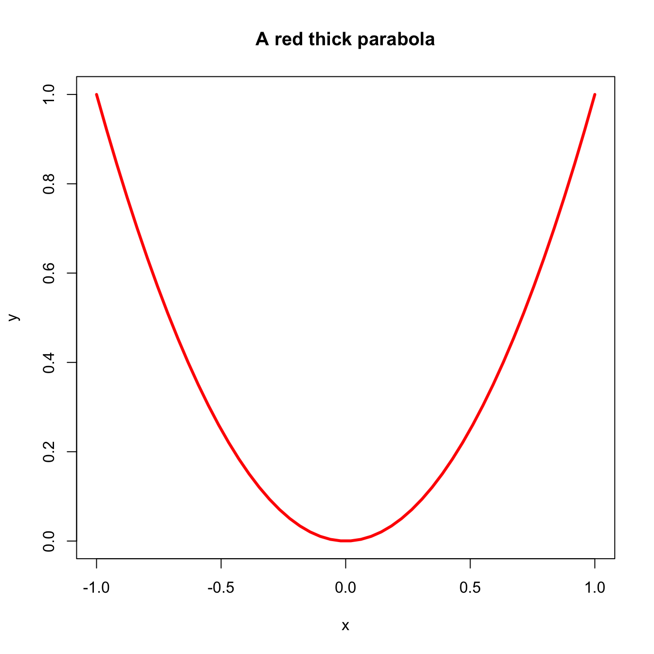
# Plotting a more complicated curve between -pi and pi
x <- seq(-pi, pi, l = 50)
y <- (2 + sin(10 * x)) * x^2
plot(x, y, type = "l") # Kind of rough...
# Remember that we are joining points for creating a curve!
# More detailed plot
x <- seq(-pi, pi, l = 500)
y <- (2 + sin(10 * x)) * x^2
plot(x, y, type = "l")
# For more options in the plot customization see
?plot
## Help on topic 'plot' was found in the following packages:
##
##   Package               Library
##   base                  /Library/Frameworks/R.framework/Resources/library
##   graphics              /Library/Frameworks/R.framework/Versions/4.2-arm64/Resources/library
##
##
## Using the first match ...
?par

# "plot" is a first level plotting function. That means that
# whenever is called, it creates a new plot. If we want to
# add information to an existing plot, we have to use a second
# level plotting function such as "points", "lines" or "abline"

plot(x, y) # Create a plot
lines(x, x^2, col = "red") # Add lines
points(x, y + 10, col = "blue") # Add points
abline(a = 5, b = 1, col = "orange", lwd = 2) # Add a straight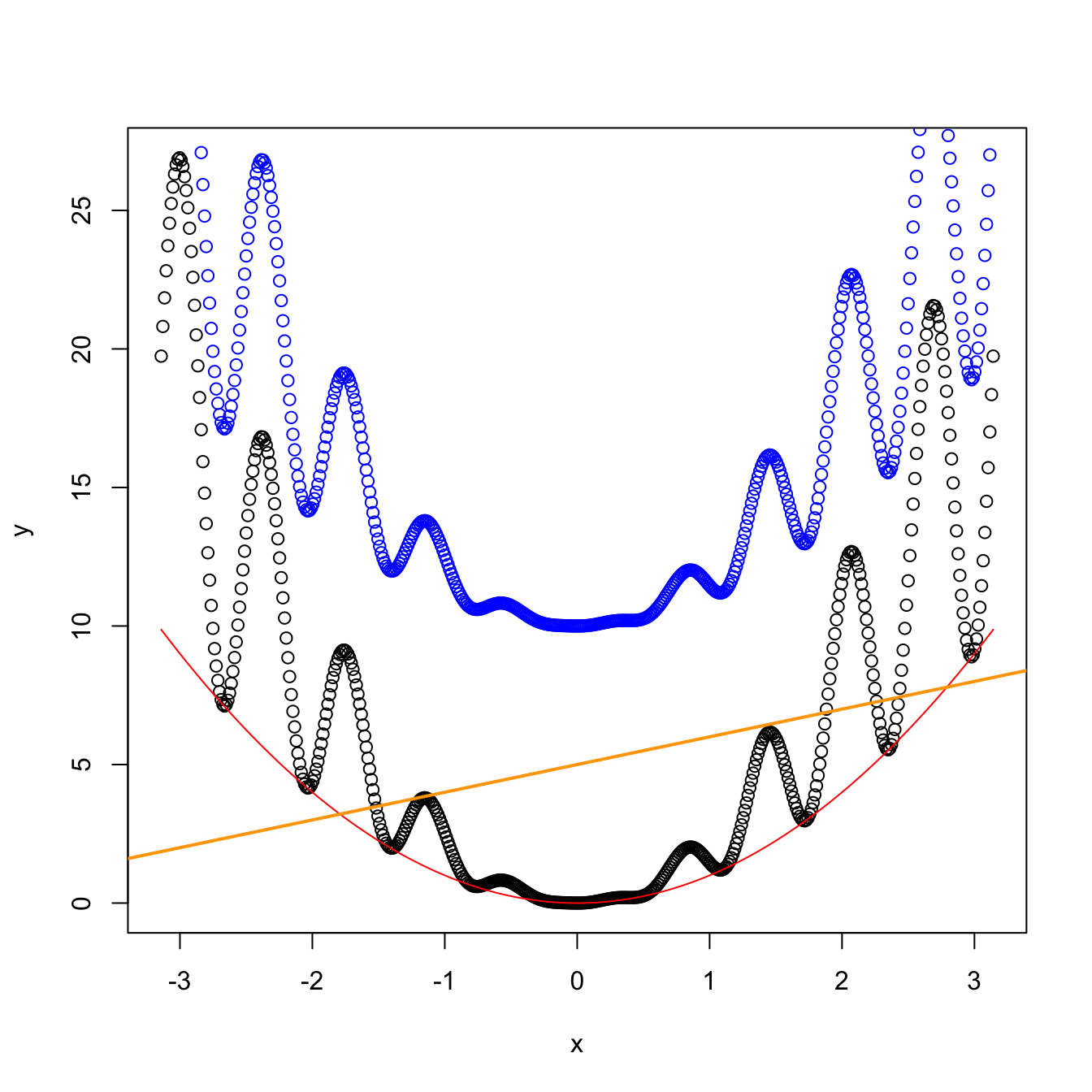
Do the following:
- Plot the
faithfuldataset. - Add the straight line \(y=110-15x\) (red).
- Make a new plot for the function \(y=\sin(x)\) (black). Add \(y=\sin(2x)\) (red), \(y=\sin(3x)\) (blue), and \(y=\sin(4x)\) (orange).
Distributions
# R allows to sample [r], compute density/probability mass
# functions [d], compute distribution function [p], and compute
# quantiles [q] for several continuous and discrete distributions.
# The format employed is [rdpq]name, where name stands for:
# - norm -> Normal
# - unif -> Uniform
# - exp -> Exponential
# - t -> Student's t
# - f -> Snedecor's F
# - chisq -> Chi squared
# - pois -> Poisson
# - binom -> Binomial
# More distributions:
?Distributions

# Sampling from a normal -- 5 random points from a N(0, 1)
rnorm(n = 5, mean = 0, sd = 1)
## [1] -0.5881703  0.3004478 -2.0931383  1.8219223  0.3728798

# If you want to have always the same result, set the seed of
# the random number generator
set.seed(45678)
rnorm(n = 5, mean = 0, sd = 1)
## [1]  1.4404800 -0.7195761  0.6709784 -0.4219485  0.3782196

# Plotting the density of a N(0, 1) -- the Gaussian bell
x <- seq(-4, 4, l = 100)
y <- dnorm(x = x, mean = 0, sd = 1)
plot(x, y, type = "l")
# Plotting the distribution function of a N(0, 1)
x <- seq(-4, 4, l = 100)
y <- pnorm(q = x, mean = 0, sd = 1)
plot(x, y, type = "l")
# Computing the 95% quantile for a N(0, 1)
qnorm(p = 0.95, mean = 0, sd = 1)
## [1] 1.644854

# All distributions have the same syntax: rname(n,...),
# dname(x,...), dname(p,...) and qname(p,...), but the
# parameters in ... change. Look them in ?Distributions
# For example, here is the same for the uniform distribution

# Sampling from a U(0, 1)
set.seed(45678)
runif(n = 10, min = 0, max = 1)
##  [1] 0.9251342 0.3339988 0.2358930 0.3366312 0.7488829 0.9327177 0.3365313 0.2245505 0.6473663 0.0807549

# Plotting the density of a U(0, 1)
x <- seq(-2, 2, l = 100)
y <- dunif(x = x, min = 0, max = 1)
plot(x, y, type = "l")
# Computing the 95% quantile for a U(0, 1)
qunif(p = 0.95, min = 0, max = 1)
## [1] 0.95

# Sampling from a Bi(10, 0.5)
set.seed(45678)
samp <- rbinom(n = 200, size = 10, prob = 0.5)
table(samp) / 200
## samp
##     1     2     3     4     5     6     7     8     9
## 0.010 0.060 0.115 0.220 0.210 0.215 0.115 0.045 0.010

# Plotting the probability mass of a Bi(10, 0.5)
x <- 0:10
y <- dbinom(x = x, size = 10, prob = 0.5)
plot(x, y, type = "h") # Vertical bars
# Plotting the distribution function of a Bi(10, 0.5)
x <- 0:10
y <- pbinom(q = x, size = 10, prob = 0.5)
plot(x, y, type = "h")
Do the following:
- Compute the \(90\%,\) \(95\%\) and \(99\%\) quantiles of a \(F\) distribution with
df1 = 1anddf2 = 5. Answer:c(4.060420, 6.607891, 16.258177). - Plot the distribution function of a \(\mathcal{U}(0,1).\) Does it make sense with its density function?
- Sample \(100\) points from a Poisson with
lambda = 5. - Sample \(100\) points from a \(\mathcal{U}(-1,1)\) and compute its mean.
- Plot the density of a \(t\) distribution with
df = 1(use a sequence spanning from-4to4). Add lines of different colors with the densities fordf = 5,df = 10,df = 50, anddf = 100. Do you see any pattern?
Functions
# A function is a way of encapsulating a block of code so it can
# be reused easily. They are useful for simplifying repetitive
# tasks and organize analyses

# This is a silly function that takes x and y and returns its sum
# Note the use of "return" to indicate what should be returned
add <- function(x, y) {
  z <- x + y
  return(z)
}

# Calling add -- you need to run the definition of the function
# first!
add(x = 1, y = 2)
## [1] 3
add(1, 1) # Arguments names can be omitted
## [1] 2

# A more complex function: computes a linear model and its
# posterior summary. Saves us a few keystrokes when computing a
# lm and a summary
lmSummary <- function(formula, data) {
  model <- lm(formula = formula, data = data)
  summary(model)
}
# If no return(), the function returns the value of the last
# expression

# Usage
lmSummary(Sepal.Length ~ Petal.Width, iris)
##
## Call:
## lm(formula = formula, data = data)
##
## Residuals:
##      Min       1Q   Median       3Q      Max
## -1.38822 -0.29358 -0.04393  0.26429  1.34521
##
## Coefficients:
##             Estimate Std. Error t value Pr(>|t|)
## (Intercept)  4.77763    0.07293   65.51   <2e-16 ***
## Petal.Width  0.88858    0.05137   17.30   <2e-16 ***
## ---
## Signif. codes:  0 '***' 0.001 '**' 0.01 '*' 0.05 '.' 0.1 ' ' 1
##
## Residual standard error: 0.478 on 148 degrees of freedom
## Multiple R-squared:  0.669,  Adjusted R-squared:  0.6668
## F-statistic: 299.2 on 1 and 148 DF,  p-value: < 2.2e-16

# Recall: there is no variable called model in the workspace.
# The function works on its own workspace!
model
## Error in eval(expr, envir, enclos): object 'model' not found

# Add a line to a plot
addLine <- function(x, beta0, beta1) {
  lines(x, beta0 + beta1 * x, lwd = 2, col = 2)
}

# Usage
plot(x, y)
addLine(x, beta0 = 0.1, beta1 = 0)
# The function "sapply" allows to sequentially apply a function
sapply(1:10, sqrt)
##  [1] 1.000000 1.414214 1.732051 2.000000 2.236068 2.449490 2.645751 2.828427 3.000000 3.162278
sqrt(1:10) # The same
##  [1] 1.000000 1.414214 1.732051 2.000000 2.236068 2.449490 2.645751 2.828427 3.000000 3.162278

# The advantage of "sapply" is that you can use with any function
myFun <- function(x) c(x, x^2)
sapply(1:10, myFun) # Returns a 2 x 10 matrix
##      [,1] [,2] [,3] [,4] [,5] [,6] [,7] [,8] [,9] [,10]
## [1,]    1    2    3    4    5    6    7    8    9    10
## [2,]    1    4    9   16   25   36   49   64   81   100

# "sapply" is useful for plotting non-vectorized functions
sumSeries <- function(n) sum(1:n)
plot(1:10, sapply(1:10, sumSeries), type = "l")
# "apply" applies iteratively a function to rows (1) or columns
# (2) of a matrix or data frame
A <- matrix(1:10, nrow = 5, ncol = 2)
A
##      [,1] [,2]
## [1,]    1    6
## [2,]    2    7
## [3,]    3    8
## [4,]    4    9
## [5,]    5   10
apply(A, 1, sum) # Applies the function by rows
## [1]  7  9 11 13 15
apply(A, 2, sum) # By columns
## [1] 15 40

# With other functions
apply(A, 1, sqrt)
##         [,1]     [,2]     [,3] [,4]     [,5]
## [1,] 1.00000 1.414214 1.732051    2 2.236068
## [2,] 2.44949 2.645751 2.828427    3 3.162278
apply(A, 2, function(x) x^2)
##      [,1] [,2]
## [1,]    1   36
## [2,]    4   49
## [3,]    9   64
## [4,]   16   81
## [5,]   25  100
Do the following:
- Create a function that takes as argument \(n\) and returns the value of \(\sum_{i=1}^n i^2.\)
- Create a function that takes as input the argument \(N\) and then plots the curve \((n, \sum_{i=1}^n \sqrt{i})\) for \(n=1,\ldots,N.\) Hint: use
sapply.
Control structures
# The "for" statement allows to create loops that run along a
# given vector
# Print 3 times a message (i varies in 1:3)
for (i in 1:3) {
  print(i)
}
## [1] 1
## [1] 2
## [1] 3

# Another example
a <- 0
for (i in 1:3) {
  a <- i + a
}
a
## [1] 6

# Nested loops are possible
A <- matrix(0, nrow = 2, ncol = 3)
for (i in 1:2) {
  for (j in 1:3) {
    A[i, j] <- i + j
  }
}

# The "if" statement allows to create conditional structures of
# the forms:
# if (condition) {
#  # Something
# } else {
#  # Something else
# }
# These structures are thought to be inside functions

# Is the number positive?
isPositive <- function(x) {
  if (x > 0) {
    print("Positive")
  } else {
    print("Not positive")
  }
}
isPositive(1)
## [1] "Positive"
isPositive(-1)
## [1] "Not positive"

# A loop can be interrupted with the "break" statement
# Stop when x is above 100
x <- 1
for (i in 1:1000) {
  x <- (x + 0.01) * x
  print(x)
  if (x > 100) {
    break
  }
}
## [1] 1.01
## [1] 1.0302
## [1] 1.071614
## [1] 1.159073
## [1] 1.35504
## [1] 1.849685
## [1] 3.439832
## [1] 11.86684
## [1] 140.9406
Do the following:
- Compute \(\mathbf{C}_{n\times k}\) in \(\mathbf{C}_{n\times k}=\mathbf{A}_{n\times m} \mathbf{B}_{m\times k}\) from \(\mathbf{A}\) and \(\mathbf{B}.\) Use that \(c_{i,j}=\sum_{\ell=1}^ma_{i,l}b_{l,j}.\) Test the implementation with simple examples.
- Create a function that samples a \(\mathcal{N}(0,1)\) and returns the first sampled point that is larger than \(4.\)
- Create a function that simulates \(N\) samples from the distribution of \(\max(X_1,\ldots,X_n)\) where \(X_1,\ldots,X_n\) are iid \(\mathcal{U}(0,1).\)