3.2 Model selection

In Chapter 2 we briefly saw that the inclusion of more predictors is not for free: there is a price to pay in terms of more variability in the coefficients estimates, harder interpretation, and possible inclusion of highly-dependent predictors. Indeed, there is a maximum number of predictors $p$ that can be considered in a linear model for a sample size $n$: \[\begin{align*} p\leq n-2. \end{align*}\] Equivalently, there is a minimum sample size $n$ required for fitting a model with $p$ predictors: $n\geq p + 2.$

The interpretation of this fact is simple if we think on the geometry for $p=1$ and $p=2$:

If $p=1,$ we need at least $n=2$ points to uniquely fit a line. However, this line gives no information on the vertical variation about it, hence $\sigma^2$ cannot be estimated⁵². Therefore, we need at least $n=3$ points, that is, $n\geq p + 2=3.$
If $p=2,$ we need at least $n=3$ points to uniquely fit a plane. But again this plane gives no information on the variation of the data about it and hence $\sigma^2$ cannot be estimated. Therefore, we need $n\geq p + 2=4.$

Another interpretation is the following:

The fitting of a linear model with $p$ predictors involves the estimation of $p+2$ parameters $(\boldsymbol{\beta},\sigma^2)$ from $n$ data points. The closer $p+2$ and $n$ are, the more variable the estimates $(\hat{\boldsymbol{\beta}},\hat\sigma^2)$ will be, since less information is available for estimating each one. In the limit case $n=p+2,$ each sample point determines a parameter estimate.

In the above discussion the degenerate case $p=n-1$ was excluded, as it gives a perfect and useless fit for which $\hat\sigma^2$ is not defined. However, $\hat{\boldsymbol{\beta}}$ is actually computable if $p=n-1.$ The output of the next chunk of code clarifies the distinction between $p=n-1$ and $p=n-2.$

# Data: n observations and p = n - 1 predictors
set.seed(123456)
n <- 5
p <- n - 1
df <- data.frame(y = rnorm(n), x = matrix(rnorm(n * p), nrow = n, ncol = p))

# Case p = n - 1 = 4: beta can be estimated, but sigma^2 cannot (hence, no
# inference can be performed since it requires the estimated sigma^2)
summary(lm(y ~ ., data = df))

# Case p = n - 2 = 3: both beta and sigma^2 can be estimated (hence, inference
# can be performed)
summary(lm(y ~ . - x.1, data = df))

The degrees of freedom $n-p-1$ quantify the increase in the variability of $(\hat{\boldsymbol{\beta}},\hat\sigma^2)$ when $p$ approaches $n-2.$ For example:

$t_{n-p-1;\alpha/2}$ appears in (2.16) and influences the length of the CIs for $\beta_j,$ see (2.17). It also influences the length of the CIs for the prediction. As Figure 3.2 shows, when the degrees of freedom decrease, $t_{n-p-1;\alpha/2}$ increases, thus the intervals widen.
$\hat\sigma^2=\frac{1}{n-p-1}\sum_{i=1}^n\hat\varepsilon_i^2$ influences the $R^2$ and $R^2_\text{Adj}.$ If no relevant variables are added to the model then $\sum_{i=1}^n\hat\varepsilon_i^2$ will not change substantially. However, the factor $\frac{1}{n-p-1}$ will increase as $p$ augments, inflating $\hat\sigma^2$ and its variance. This is exactly what happened in Figure 2.19.

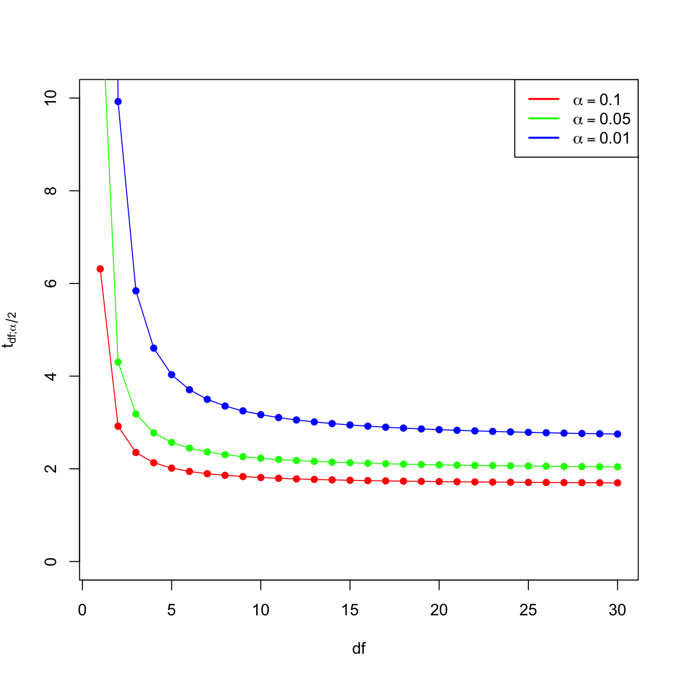
$Effect of $\text{df}=n-p-1$ in $t_{\text{df};\alpha/2}$ for $\alpha=0.10,0.05,0.01.$$

Figure 3.2: Effect of $\text{df}=n-p-1$ in $t_{\text{df};\alpha/2}$ for $\alpha=0.10,0.05,0.01.$

Now that we have shed more light on the problem of having an excess of predictors, we turn the focus on selecting the most adequate predictors for a multiple regression model. This is a challenging task without a unique solution, and what is worse, without a method that is guaranteed to work in all the cases. However, there is a well-established procedure that usually gives good results: the stepwise model selection. Its principle is to sequentially compare multiple linear regression models with different predictors⁵³, improving iteratively a performance measure through a greedy search.

Stepwise model selection typically uses as measure of performance an information criterion. An information criterion balances the fitness of a model with the number of predictors employed. Hence, it determines objectively the best model as the one that minimizes the considered information criterion. Two common criteria are the Bayesian Information Criterion (BIC) and the Akaike Information Criterion (AIC). Both are based on balancing the model fitness and its complexity:

\[\begin{align} \text{BIC}(\text{model}) = \underbrace{-2\ell(\text{model})}_{\text{Model fitness}} + \underbrace{\text{npar(model)}\times\log(n)}_{\text{Complexity}}, \tag{3.1} \end{align}\]

where $\ell(\text{model})$ is the log-likelihood of the model (how well the model fits the data) and $\text{npar(model)}$ is the number of parameters considered in the model (how complex the model is). In the case of a multiple linear regression model with $p$ predictors, $\text{npar(model)}=p+2.$ The AIC replaces the $\log(n)$ factor by a $2$ in (3.1) so, compared with the BIC, it penalizes less the more complex models⁵⁴. This is one of the reasons why BIC is preferred by some practitioners for performing model comparison⁵⁵.

The BIC and AIC can be computed through the functions BIC and AIC. They take a model as the input.

# Two models with different predictors
mod1 <- lm(medv ~ age + crim, data = Boston)
mod2 <- lm(medv ~ age + crim + lstat, data = Boston)

# BICs
BIC(mod1)
## [1] 3581.893
BIC(mod2) # Smaller -> better
## [1] 3300.841

# AICs
AIC(mod1)
## [1] 3564.987
AIC(mod2) # Smaller -> better
## [1] 3279.708

# Check the summaries
summary(mod1)
## 
## Call:
## lm(formula = medv ~ age + crim, data = Boston)
## 
## Residuals:
##     Min      1Q  Median      3Q     Max 
## -13.940  -4.991  -2.420   2.110  32.033 
## 
## Coefficients:
##             Estimate Std. Error t value Pr(>|t|)    
## (Intercept) 29.80067    0.97078  30.698  < 2e-16 ***
## age         -0.08955    0.01378  -6.499 1.95e-10 ***
## crim        -0.31182    0.04510  -6.914 1.43e-11 ***
## ---
## Signif. codes:  0 '***' 0.001 '**' 0.01 '*' 0.05 '.' 0.1 ' ' 1
## 
## Residual standard error: 8.157 on 503 degrees of freedom
## Multiple R-squared:  0.2166, Adjusted R-squared:  0.2134 
## F-statistic: 69.52 on 2 and 503 DF,  p-value: < 2.2e-16
summary(mod2)
## 
## Call:
## lm(formula = medv ~ age + crim + lstat, data = Boston)
## 
## Residuals:
##     Min      1Q  Median      3Q     Max 
## -16.133  -3.848  -1.380   1.970  23.644 
## 
## Coefficients:
##             Estimate Std. Error t value Pr(>|t|)    
## (Intercept) 32.82804    0.74774  43.903  < 2e-16 ***
## age          0.03765    0.01225   3.074  0.00223 ** 
## crim        -0.08262    0.03594  -2.299  0.02193 *  
## lstat       -0.99409    0.05075 -19.587  < 2e-16 ***
## ---
## Signif. codes:  0 '***' 0.001 '**' 0.01 '*' 0.05 '.' 0.1 ' ' 1
## 
## Residual standard error: 6.147 on 502 degrees of freedom
## Multiple R-squared:  0.5559, Adjusted R-squared:  0.5533 
## F-statistic: 209.5 on 3 and 502 DF,  p-value: < 2.2e-16

Let’s go back to the selection of predictors. If we have $p$ predictors, a naive procedure would be to check all the possible models that can be constructed with them and then select the best one in terms of BIC/AIC. This exhaustive search is the so-called best subset selection – its application to be seen in Section 4.4. The problem is that there are $2^p$ possible models to inspect!⁵⁶ Fortunately, the MASS::stepAIC function helps us navigating this ocean of models by implementing stepwise model selection. Stepwise selection will iteratively add predictors that decrease an information criterion and/or remove those that increase it, depending on the mode of stepwise search that is performed.

stepAIC takes as input an initial model to be improved and has several variants. Let’s see first how it works in its default mode using the already studied wine dataset.

# Load data -- notice that "Year" is also included
wine <- read.csv(file = "wine.csv", header = TRUE)

We use as initial model the one featuring all the available predictors. The argument k of stepAIC stands for the factor post-multiplying $\text{npar(model)}$ in (3.1). It defaults to $2,$ which gives the AIC. If we set it to k = log(n), the function considers the BIC.

# Full model
mod <- lm(Price ~ ., data = wine)

# With AIC
modAIC <- MASS::stepAIC(mod, k = 2)
## Start:  AIC=-61.07
## Price ~ Year + WinterRain + AGST + HarvestRain + Age + FrancePop
## 
## 
## Step:  AIC=-61.07
## Price ~ Year + WinterRain + AGST + HarvestRain + FrancePop
## 
##               Df Sum of Sq    RSS     AIC
## - FrancePop    1    0.0026 1.8058 -63.031
## - Year         1    0.0048 1.8080 -62.998
## <none>                     1.8032 -61.070
## - WinterRain   1    0.4585 2.2617 -56.952
## - HarvestRain  1    1.8063 3.6095 -44.331
## - AGST         1    3.3756 5.1788 -34.584
## 
## Step:  AIC=-63.03
## Price ~ Year + WinterRain + AGST + HarvestRain
## 
##               Df Sum of Sq    RSS     AIC
## <none>                     1.8058 -63.031
## - WinterRain   1    0.4809 2.2867 -58.656
## - Year         1    0.9089 2.7147 -54.023
## - HarvestRain  1    1.8760 3.6818 -45.796
## - AGST         1    3.4428 5.2486 -36.222

# The result is an lm object
summary(modAIC)
## 
## Call:
## lm(formula = Price ~ Year + WinterRain + AGST + HarvestRain, 
##     data = wine)
## 
## Residuals:
##      Min       1Q   Median       3Q      Max 
## -0.46024 -0.23862  0.01347  0.18601  0.53443 
## 
## Coefficients:
##               Estimate Std. Error t value Pr(>|t|)    
## (Intercept) 43.6390418 14.6939240   2.970  0.00707 ** 
## Year        -0.0238480  0.0071667  -3.328  0.00305 ** 
## WinterRain   0.0011667  0.0004820   2.420  0.02421 *  
## AGST         0.6163916  0.0951747   6.476 1.63e-06 ***
## HarvestRain -0.0038606  0.0008075  -4.781 8.97e-05 ***
## ---
## Signif. codes:  0 '***' 0.001 '**' 0.01 '*' 0.05 '.' 0.1 ' ' 1
## 
## Residual standard error: 0.2865 on 22 degrees of freedom
## Multiple R-squared:  0.8275, Adjusted R-squared:  0.7962 
## F-statistic: 26.39 on 4 and 22 DF,  p-value: 4.057e-08

# With BIC
modBIC <- MASS::stepAIC(mod, k = log(nrow(wine)))
## Start:  AIC=-53.29
## Price ~ Year + WinterRain + AGST + HarvestRain + Age + FrancePop
## 
## 
## Step:  AIC=-53.29
## Price ~ Year + WinterRain + AGST + HarvestRain + FrancePop
## 
##               Df Sum of Sq    RSS     AIC
## - FrancePop    1    0.0026 1.8058 -56.551
## - Year         1    0.0048 1.8080 -56.519
## <none>                     1.8032 -53.295
## - WinterRain   1    0.4585 2.2617 -50.473
## - HarvestRain  1    1.8063 3.6095 -37.852
## - AGST         1    3.3756 5.1788 -28.105
## 
## Step:  AIC=-56.55
## Price ~ Year + WinterRain + AGST + HarvestRain
## 
##               Df Sum of Sq    RSS     AIC
## <none>                     1.8058 -56.551
## - WinterRain   1    0.4809 2.2867 -53.473
## - Year         1    0.9089 2.7147 -48.840
## - HarvestRain  1    1.8760 3.6818 -40.612
## - AGST         1    3.4428 5.2486 -31.039

An explanation of what stepAIC did for modBIC:

At each step, stepAIC displayed information about the current value of the information criterion. For example, the BIC at the first step was Step: AIC=-53.29 and then it improved to Step: AIC=-56.55 in the second step.⁵⁷
The next model to move on was decided by exploring the information criteria of the different models resulting from adding or removing a predictor (depending on the direction argument, explained later). For example, in the first step the model arising from removing⁵⁸ FrancePop had a BIC equal to -56.551.
The stepwise regression proceeded then by removing FrancePop, as it gave the lowest BIC. When repeating the previous exploration, it was found that removing <none> predictors was the best possible action.

The selected models modBIC and modAIC are equivalent to the modWine2 we selected in Section 2.7.3 as the best model. This is a simple illustration that the model selected by stepAIC is often a good starting point for further additions or deletions of predictors.

The direction argument of stepAIC controls the mode of the stepwise model search:

"backward": removes predictors sequentially from the given model. It produces a sequence of models of decreasing complexity until attaining the optimal one.
"forward": adds predictors sequentially to the given model, using the available ones in the data argument of lm. It produces a sequence of models of increasing complexity until attaining the optimal one.
"both" (default): a forward-backward search that, at each step, decides whether to include or exclude a predictor. Differently from the previous modes, a predictor that was excluded/included previously can be later included/excluded.

The next chunk of code clearly explains how to exploit the direction argument, and other options of stepAIC, with a modified version of the wine dataset. An important warning is that in order to use direction = "forward" or direction = "both", scope needs to be properly defined. The practical advice to model selection is to run⁵⁹ several of these three search modes and retain the model with minimum BIC/AIC, being specially careful with the scope argument.

# Add an irrelevant predictor to the wine dataset
set.seed(123456)
wineNoise <- wine
n <- nrow(wineNoise)
wineNoise$noisePredictor <- rnorm(n)

# Backward selection: removes predictors sequentially from the given model

# Starting from the model with all the predictors
modAll <- lm(formula = Price ~ ., data = wineNoise)
MASS::stepAIC(modAll, direction = "backward", k = log(n))
## Start:  AIC=-50.13
## Price ~ Year + WinterRain + AGST + HarvestRain + Age + FrancePop + 
##     noisePredictor
## 
## 
## Step:  AIC=-50.13
## Price ~ Year + WinterRain + AGST + HarvestRain + FrancePop + 
##     noisePredictor
## 
##                  Df Sum of Sq    RSS     AIC
## - FrancePop       1    0.0036 1.7977 -53.376
## - Year            1    0.0038 1.7979 -53.374
## - noisePredictor  1    0.0090 1.8032 -53.295
## <none>                        1.7941 -50.135
## - WinterRain      1    0.4598 2.2539 -47.271
## - HarvestRain     1    1.7666 3.5607 -34.923
## - AGST            1    3.3658 5.1599 -24.908
## 
## Step:  AIC=-53.38
## Price ~ Year + WinterRain + AGST + HarvestRain + noisePredictor
## 
##                  Df Sum of Sq    RSS     AIC
## - noisePredictor  1    0.0081 1.8058 -56.551
## <none>                        1.7977 -53.376
## - WinterRain      1    0.4771 2.2748 -50.317
## - Year            1    0.9162 2.7139 -45.552
## - HarvestRain     1    1.8449 3.6426 -37.606
## - AGST            1    3.4234 5.2212 -27.885
## 
## Step:  AIC=-56.55
## Price ~ Year + WinterRain + AGST + HarvestRain
## 
##               Df Sum of Sq    RSS     AIC
## <none>                     1.8058 -56.551
## - WinterRain   1    0.4809 2.2867 -53.473
## - Year         1    0.9089 2.7147 -48.840
## - HarvestRain  1    1.8760 3.6818 -40.612
## - AGST         1    3.4428 5.2486 -31.039
## 
## Call:
## lm(formula = Price ~ Year + WinterRain + AGST + HarvestRain, 
##     data = wineNoise)
## 
## Coefficients:
## (Intercept)         Year   WinterRain         AGST  HarvestRain  
##   43.639042    -0.023848     0.001167     0.616392    -0.003861

# Starting from an intermediate model
modInter <- lm(formula = Price ~ noisePredictor + Year + AGST, data = wineNoise)
MASS::stepAIC(modInter, direction = "backward", k = log(n))
## Start:  AIC=-32.38
## Price ~ noisePredictor + Year + AGST
## 
##                  Df Sum of Sq    RSS     AIC
## - noisePredictor  1    0.0146 5.0082 -35.601
## <none>                        4.9936 -32.384
## - Year            1    0.7522 5.7459 -31.891
## - AGST            1    3.2211 8.2147 -22.240
## 
## Step:  AIC=-35.6
## Price ~ Year + AGST
## 
##        Df Sum of Sq    RSS     AIC
## <none>              5.0082 -35.601
## - Year  1    0.7966 5.8049 -34.911
## - AGST  1    3.2426 8.2509 -25.417
## 
## Call:
## lm(formula = Price ~ Year + AGST, data = wineNoise)
## 
## Coefficients:
## (Intercept)         Year         AGST  
##    41.49441     -0.02221      0.56067
# Recall that other predictors not included in modInter are not explored
# during the search (so the relevant predictor HarvestRain is not added)

# Forward selection: adds predictors sequentially from the given model

# Starting from the model with no predictors, only intercept (denoted as ~ 1)
modZero <- lm(formula = Price ~ 1, data = wineNoise)
MASS::stepAIC(modZero, direction = "forward",
              scope = list(lower = modZero, upper = modAll), k = log(n))
## Start:  AIC=-22.28
## Price ~ 1
## 
##                  Df Sum of Sq     RSS     AIC
## + AGST            1    4.6655  5.8049 -34.911
## + HarvestRain     1    2.6933  7.7770 -27.014
## + FrancePop       1    2.4231  8.0472 -26.092
## + Year            1    2.2195  8.2509 -25.417
## + Age             1    2.2195  8.2509 -25.417
## <none>                        10.4703 -22.281
## + WinterRain      1    0.1905 10.2798 -19.481
## + noisePredictor  1    0.1761 10.2942 -19.443
## 
## Step:  AIC=-34.91
## Price ~ AGST
## 
##                  Df Sum of Sq    RSS     AIC
## + HarvestRain     1   2.50659 3.2983 -46.878
## + WinterRain      1   1.42392 4.3809 -39.214
## + FrancePop       1   0.90263 4.9022 -36.178
## + Year            1   0.79662 5.0082 -35.601
## + Age             1   0.79662 5.0082 -35.601
## <none>                        5.8049 -34.911
## + noisePredictor  1   0.05900 5.7459 -31.891
## 
## Step:  AIC=-46.88
## Price ~ AGST + HarvestRain
## 
##                  Df Sum of Sq    RSS     AIC
## + FrancePop       1   1.03572 2.2625 -53.759
## + Year            1   1.01159 2.2867 -53.473
## + Age             1   1.01159 2.2867 -53.473
## + WinterRain      1   0.58356 2.7147 -48.840
## <none>                        3.2983 -46.878
## + noisePredictor  1   0.06084 3.2374 -44.085
## 
## Step:  AIC=-53.76
## Price ~ AGST + HarvestRain + FrancePop
## 
##                  Df Sum of Sq    RSS     AIC
## + WinterRain      1   0.45456 1.8080 -56.519
## <none>                        2.2625 -53.759
## + noisePredictor  1   0.00829 2.2542 -50.562
## + Year            1   0.00085 2.2617 -50.473
## + Age             1   0.00085 2.2617 -50.473
## 
## Step:  AIC=-56.52
## Price ~ AGST + HarvestRain + FrancePop + WinterRain
## 
##                  Df Sum of Sq    RSS     AIC
## <none>                        1.8080 -56.519
## + noisePredictor  1 0.0100635 1.7979 -53.374
## + Year            1 0.0048039 1.8032 -53.295
## + Age             1 0.0048039 1.8032 -53.295
## 
## Call:
## lm(formula = Price ~ AGST + HarvestRain + FrancePop + WinterRain, 
##     data = wineNoise)
## 
## Coefficients:
## (Intercept)         AGST  HarvestRain    FrancePop   WinterRain  
##  -5.945e-01    6.127e-01   -3.804e-03   -5.189e-05    1.136e-03
# It is very important to set the scope argument adequately when doing forward
# search! In the scope you have to define the "minimum" (lower) and "maximum"
# (upper) models that contain the set of explorable models. If not provided,
# the maximum model will be taken as the passed starting model (in this case
# modZero) and stepAIC will not do any search

# Starting from an intermediate model
MASS::stepAIC(modInter, direction = "forward",
              scope = list(lower = modZero, upper = modAll), k = log(n))
## Start:  AIC=-32.38
## Price ~ noisePredictor + Year + AGST
## 
##               Df Sum of Sq    RSS     AIC
## + HarvestRain  1   2.71878 2.2748 -50.317
## + WinterRain   1   1.35102 3.6426 -37.606
## <none>                     4.9936 -32.384
## + FrancePop    1   0.24004 4.7536 -30.418
## 
## Step:  AIC=-50.32
## Price ~ noisePredictor + Year + AGST + HarvestRain
## 
##              Df Sum of Sq    RSS     AIC
## + WinterRain  1   0.47710 1.7977 -53.376
## <none>                    2.2748 -50.317
## + FrancePop   1   0.02094 2.2539 -47.271
## 
## Step:  AIC=-53.38
## Price ~ noisePredictor + Year + AGST + HarvestRain + WinterRain
## 
##             Df Sum of Sq    RSS     AIC
## <none>                   1.7977 -53.376
## + FrancePop  1 0.0036037 1.7941 -50.135
## 
## Call:
## lm(formula = Price ~ noisePredictor + Year + AGST + HarvestRain + 
##     WinterRain, data = wineNoise)
## 
## Coefficients:
##    (Intercept)  noisePredictor            Year            AGST     HarvestRain      WinterRain  
##      44.096639       -0.019617       -0.024126        0.620522       -0.003840        0.001211
# Recall that predictors included in modInter are not dropped during the
# search (so the irrelevant noisePredictor is kept)

# Both selection: useful if starting from an intermediate model

# Removes the problems associated to "backward" and "forward" searches done
# from intermediate models
MASS::stepAIC(modInter, direction = "both",
              scope = list(lower = modZero, upper = modAll), k = log(n))
## Start:  AIC=-32.38
## Price ~ noisePredictor + Year + AGST
## 
##                  Df Sum of Sq    RSS     AIC
## + HarvestRain     1    2.7188 2.2748 -50.317
## + WinterRain      1    1.3510 3.6426 -37.606
## - noisePredictor  1    0.0146 5.0082 -35.601
## <none>                        4.9936 -32.384
## - Year            1    0.7522 5.7459 -31.891
## + FrancePop       1    0.2400 4.7536 -30.418
## - AGST            1    3.2211 8.2147 -22.240
## 
## Step:  AIC=-50.32
## Price ~ noisePredictor + Year + AGST + HarvestRain
## 
##                  Df Sum of Sq    RSS     AIC
## - noisePredictor  1   0.01182 2.2867 -53.473
## + WinterRain      1   0.47710 1.7977 -53.376
## <none>                        2.2748 -50.317
## + FrancePop       1   0.02094 2.2539 -47.271
## - Year            1   0.96258 3.2374 -44.085
## - HarvestRain     1   2.71878 4.9936 -32.384
## - AGST            1   2.94647 5.2213 -31.180
## 
## Step:  AIC=-53.47
## Price ~ Year + AGST + HarvestRain
## 
##                  Df Sum of Sq    RSS     AIC
## + WinterRain      1   0.48087 1.8058 -56.551
## <none>                        2.2867 -53.473
## + FrancePop       1   0.02497 2.2617 -50.473
## + noisePredictor  1   0.01182 2.2748 -50.317
## - Year            1   1.01159 3.2983 -46.878
## - HarvestRain     1   2.72157 5.0082 -35.601
## - AGST            1   2.96500 5.2517 -34.319
## 
## Step:  AIC=-56.55
## Price ~ Year + AGST + HarvestRain + WinterRain
## 
##                  Df Sum of Sq    RSS     AIC
## <none>                        1.8058 -56.551
## - WinterRain      1    0.4809 2.2867 -53.473
## + noisePredictor  1    0.0081 1.7977 -53.376
## + FrancePop       1    0.0026 1.8032 -53.295
## - Year            1    0.9089 2.7147 -48.840
## - HarvestRain     1    1.8760 3.6818 -40.612
## - AGST            1    3.4428 5.2486 -31.039
## 
## Call:
## lm(formula = Price ~ Year + AGST + HarvestRain + WinterRain, 
##     data = wineNoise)
## 
## Coefficients:
## (Intercept)         Year         AGST  HarvestRain   WinterRain  
##   43.639042    -0.023848     0.616392    -0.003861     0.001167
# It is very important as well to correctly define the scope, because "both"
# resorts to "forward" (as well as to "backward")

# Using the defaults from the full model essentially does backward selection,
# but allowing predictors that were removed to enter again at later steps
MASS::stepAIC(modAll, direction = "both", k = log(n))
## Start:  AIC=-50.13
## Price ~ Year + WinterRain + AGST + HarvestRain + Age + FrancePop + 
##     noisePredictor
## 
## 
## Step:  AIC=-50.13
## Price ~ Year + WinterRain + AGST + HarvestRain + FrancePop + 
##     noisePredictor
## 
##                  Df Sum of Sq    RSS     AIC
## - FrancePop       1    0.0036 1.7977 -53.376
## - Year            1    0.0038 1.7979 -53.374
## - noisePredictor  1    0.0090 1.8032 -53.295
## <none>                        1.7941 -50.135
## - WinterRain      1    0.4598 2.2539 -47.271
## - HarvestRain     1    1.7666 3.5607 -34.923
## - AGST            1    3.3658 5.1599 -24.908
## 
## Step:  AIC=-53.38
## Price ~ Year + WinterRain + AGST + HarvestRain + noisePredictor
## 
##                  Df Sum of Sq    RSS     AIC
## - noisePredictor  1    0.0081 1.8058 -56.551
## <none>                        1.7977 -53.376
## - WinterRain      1    0.4771 2.2748 -50.317
## + FrancePop       1    0.0036 1.7941 -50.135
## - Year            1    0.9162 2.7139 -45.552
## - HarvestRain     1    1.8449 3.6426 -37.606
## - AGST            1    3.4234 5.2212 -27.885
## 
## Step:  AIC=-56.55
## Price ~ Year + WinterRain + AGST + HarvestRain
## 
##                  Df Sum of Sq    RSS     AIC
## <none>                        1.8058 -56.551
## - WinterRain      1    0.4809 2.2867 -53.473
## + noisePredictor  1    0.0081 1.7977 -53.376
## + FrancePop       1    0.0026 1.8032 -53.295
## - Year            1    0.9089 2.7147 -48.840
## - HarvestRain     1    1.8760 3.6818 -40.612
## - AGST            1    3.4428 5.2486 -31.039
## 
## Call:
## lm(formula = Price ~ Year + WinterRain + AGST + HarvestRain, 
##     data = wineNoise)
## 
## Coefficients:
## (Intercept)         Year   WinterRain         AGST  HarvestRain  
##   43.639042    -0.023848     0.001167     0.616392    -0.003861

# Omit lengthy outputs
MASS::stepAIC(modAll, direction = "both", trace = 0,
              scope = list(lower = modZero, upper = modAll), k = log(n))
## 
## Call:
## lm(formula = Price ~ Year + WinterRain + AGST + HarvestRain, 
##     data = wineNoise)
## 
## Coefficients:
## (Intercept)         Year   WinterRain         AGST  HarvestRain  
##   43.639042    -0.023848     0.001167     0.616392    -0.003861

Run the previous stepwise selections for the Boston dataset, with the aim of clearly understanding the different search directions. Specifically:

Do a "forward" stepwise fit starting from medv ~ 1.
Do a "forward" stepwise fit starting from medv ~ crim + lstat + age.
Do a "both" stepwise fit starting from medv ~ crim + lstat + age.
Do a "both" stepwise fit starting from medv ~ ..
Do a "backward" stepwise fit starting from medv ~ ..

We conclude with a couple of quirks of stepAIC to be aware of.

stepAIC assumes that no NA’s (missing values) are present in the data. It is advised to remove the missing values in the data before. Their presence might lead to errors. To do so, employ data = na.omit(dataset) in the call to lm (if your dataset is dataset). Also, see Appendix A.4 for possible alternatives to deal with missing data.

stepAIC and friends (addterm and dropterm) compute a slightly different version of the BIC/AIC than the BIC/AIC functions. Precisely, the BIC/AIC they report come from the extractAIC function, which differs in an additive constant from the output of BIC/AIC. This is not relevant for model comparison, since shifting by a common constant the BIC/AIC does not change the lower-to-higher BIC/AIC ordering of models. However, it is important to be aware of this fact in order to do not compare directly the output of stepAIC with the one of BIC/AIC. The additive constant (included in BIC/AIC but not in extractAIC) is $n(\log(2 \pi) + 1) + \log(n)$ for the BIC and $n(\log(2 \pi) + 1) + 2$ for the AIC. The discrepancy arises from simplifying the computation of the BIC/AIC for linear models and from counting $\hat\sigma^2$ as an estimated parameter.

The following chunk of code illustrates the relation of the AIC reported in stepsAIC, the output of extractAIC, and the BIC/AIC reported by BIC/AIC.

# Same BICs, different scale
n <- nobs(modBIC)
extractAIC(modBIC, k = log(n))[2]
## [1] -56.55135
BIC(modBIC)
## [1] 23.36717
# Observe that MASS::stepAIC(mod, k = log(nrow(wine))) returned as final BIC
# the one given by extractAIC(), not by BIC()! But both are equivalent, they
# just differ in a constant shift

# Same AICs, different scale
extractAIC(modAIC, k = 2)[2]
## [1] -63.03053
AIC(modAIC)
## [1] 15.59215

# The additive constant: BIC() includes it but extractAIC() does not
BIC(modBIC) - extractAIC(modBIC, k = log(n))[2]
## [1] 79.91852
n * (log(2 * pi) + 1) + log(n)
## [1] 79.91852

# Same for the AIC
AIC(modAIC) - extractAIC(modAIC)[2]
## [1] 78.62268
n * (log(2 * pi) + 1) + 2
## [1] 78.62268

3.2.1 Case study application

We want to build a linear model for predicting and explaining medv. There are a good number of predictors and some of them might be of little use for predicting medv. However, there is no clear intuition of which predictors will yield better explanations of medv with the information at hand. Therefore, we can start by doing a linear model on all the predictors:

modHouse <- lm(medv ~ ., data = Boston)
summary(modHouse)
## 
## Call:
## lm(formula = medv ~ ., data = Boston)
## 
## Residuals:
##     Min      1Q  Median      3Q     Max 
## -15.595  -2.730  -0.518   1.777  26.199 
## 
## Coefficients:
##               Estimate Std. Error t value Pr(>|t|)    
## (Intercept)  3.646e+01  5.103e+00   7.144 3.28e-12 ***
## crim        -1.080e-01  3.286e-02  -3.287 0.001087 ** 
## zn           4.642e-02  1.373e-02   3.382 0.000778 ***
## indus        2.056e-02  6.150e-02   0.334 0.738288    
## chas         2.687e+00  8.616e-01   3.118 0.001925 ** 
## nox         -1.777e+01  3.820e+00  -4.651 4.25e-06 ***
## rm           3.810e+00  4.179e-01   9.116  < 2e-16 ***
## age          6.922e-04  1.321e-02   0.052 0.958229    
## dis         -1.476e+00  1.995e-01  -7.398 6.01e-13 ***
## rad          3.060e-01  6.635e-02   4.613 5.07e-06 ***
## tax         -1.233e-02  3.760e-03  -3.280 0.001112 ** 
## ptratio     -9.527e-01  1.308e-01  -7.283 1.31e-12 ***
## black        9.312e-03  2.686e-03   3.467 0.000573 ***
## lstat       -5.248e-01  5.072e-02 -10.347  < 2e-16 ***
## ---
## Signif. codes:  0 '***' 0.001 '**' 0.01 '*' 0.05 '.' 0.1 ' ' 1
## 
## Residual standard error: 4.745 on 492 degrees of freedom
## Multiple R-squared:  0.7406, Adjusted R-squared:  0.7338 
## F-statistic: 108.1 on 13 and 492 DF,  p-value: < 2.2e-16

There are a couple of non-significant variables, but so far the model has an $R^2=0.74$ and the fitted coefficients are sensible with what would be expected. For example, crim, tax, ptratio, and nox have negative effects on medv, while rm, rad, and chas have positive effects. However, the non-significant coefficients are only adding noise to the prediction and decreasing the overall accuracy of the coefficient estimates.

Let’s polish the previous model a little bit. Instead of manually removing each non-significant variable to reduce the complexity, we employ stepAIC for performing a forward-backward search starting from the full model. This gives us a candidate best model.

# Best BIC and AIC models
modBIC <- MASS::stepAIC(modHouse, k = log(nrow(Boston)))
## Start:  AIC=1648.81
## medv ~ crim + zn + indus + chas + nox + rm + age + dis + rad + 
##     tax + ptratio + black + lstat
## 
##           Df Sum of Sq   RSS    AIC
## - age      1      0.06 11079 1642.6
## - indus    1      2.52 11081 1642.7
## <none>                 11079 1648.8
## - chas     1    218.97 11298 1652.5
## - tax      1    242.26 11321 1653.5
## - crim     1    243.22 11322 1653.6
## - zn       1    257.49 11336 1654.2
## - black    1    270.63 11349 1654.8
## - rad      1    479.15 11558 1664.0
## - nox      1    487.16 11566 1664.4
## - ptratio  1   1194.23 12273 1694.4
## - dis      1   1232.41 12311 1696.0
## - rm       1   1871.32 12950 1721.6
## - lstat    1   2410.84 13490 1742.2
## 
## Step:  AIC=1642.59
## medv ~ crim + zn + indus + chas + nox + rm + dis + rad + tax + 
##     ptratio + black + lstat
## 
##           Df Sum of Sq   RSS    AIC
## - indus    1      2.52 11081 1636.5
## <none>                 11079 1642.6
## - chas     1    219.91 11299 1646.3
## - tax      1    242.24 11321 1647.3
## - crim     1    243.20 11322 1647.3
## - zn       1    260.32 11339 1648.1
## - black    1    272.26 11351 1648.7
## - rad      1    481.09 11560 1657.9
## - nox      1    520.87 11600 1659.6
## - ptratio  1   1200.23 12279 1688.4
## - dis      1   1352.26 12431 1694.6
## - rm       1   1959.55 13038 1718.8
## - lstat    1   2718.88 13798 1747.4
## 
## Step:  AIC=1636.48
## medv ~ crim + zn + chas + nox + rm + dis + rad + tax + ptratio + 
##     black + lstat
## 
##           Df Sum of Sq   RSS    AIC
## <none>                 11081 1636.5
## - chas     1    227.21 11309 1640.5
## - crim     1    245.37 11327 1641.3
## - zn       1    257.82 11339 1641.9
## - black    1    270.82 11352 1642.5
## - tax      1    273.62 11355 1642.6
## - rad      1    500.92 11582 1652.6
## - nox      1    541.91 11623 1654.4
## - ptratio  1   1206.45 12288 1682.5
## - dis      1   1448.94 12530 1692.4
## - rm       1   1963.66 13045 1712.8
## - lstat    1   2723.48 13805 1741.5
modAIC <- MASS::stepAIC(modHouse, trace = 0, k = 2)

# Comparison: same fits
car::compareCoefs(modBIC, modAIC)
## Calls:
## 1: lm(formula = medv ~ crim + zn + chas + nox + rm + dis + rad + tax + ptratio + black + lstat, data = Boston)
## 2: lm(formula = medv ~ crim + zn + chas + nox + rm + dis + rad + tax + ptratio + black + lstat, data = Boston)
## 
##              Model 1  Model 2
## (Intercept)    36.34    36.34
## SE              5.07     5.07
##                              
## crim         -0.1084  -0.1084
## SE            0.0328   0.0328
##                              
## zn            0.0458   0.0458
## SE            0.0135   0.0135
##                              
## chas           2.719    2.719
## SE             0.854    0.854
##                              
## nox           -17.38   -17.38
## SE              3.54     3.54
##                              
## rm             3.802    3.802
## SE             0.406    0.406
##                              
## dis           -1.493   -1.493
## SE             0.186    0.186
##                              
## rad           0.2996   0.2996
## SE            0.0634   0.0634
##                              
## tax         -0.01178 -0.01178
## SE           0.00337  0.00337
##                              
## ptratio       -0.947   -0.947
## SE             0.129    0.129
##                              
## black        0.00929  0.00929
## SE           0.00267  0.00267
##                              
## lstat        -0.5226  -0.5226
## SE            0.0474   0.0474
## 
summary(modBIC)
## 
## Call:
## lm(formula = medv ~ crim + zn + chas + nox + rm + dis + rad + 
##     tax + ptratio + black + lstat, data = Boston)
## 
## Residuals:
##      Min       1Q   Median       3Q      Max 
## -15.5984  -2.7386  -0.5046   1.7273  26.2373 
## 
## Coefficients:
##               Estimate Std. Error t value Pr(>|t|)    
## (Intercept)  36.341145   5.067492   7.171 2.73e-12 ***
## crim         -0.108413   0.032779  -3.307 0.001010 ** 
## zn            0.045845   0.013523   3.390 0.000754 ***
## chas          2.718716   0.854240   3.183 0.001551 ** 
## nox         -17.376023   3.535243  -4.915 1.21e-06 ***
## rm            3.801579   0.406316   9.356  < 2e-16 ***
## dis          -1.492711   0.185731  -8.037 6.84e-15 ***
## rad           0.299608   0.063402   4.726 3.00e-06 ***
## tax          -0.011778   0.003372  -3.493 0.000521 ***
## ptratio      -0.946525   0.129066  -7.334 9.24e-13 ***
## black         0.009291   0.002674   3.475 0.000557 ***
## lstat        -0.522553   0.047424 -11.019  < 2e-16 ***
## ---
## Signif. codes:  0 '***' 0.001 '**' 0.01 '*' 0.05 '.' 0.1 ' ' 1
## 
## Residual standard error: 4.736 on 494 degrees of freedom
## Multiple R-squared:  0.7406, Adjusted R-squared:  0.7348 
## F-statistic: 128.2 on 11 and 494 DF,  p-value: < 2.2e-16

# Confidence intervals
confint(modBIC)
##                     2.5 %       97.5 %
## (Intercept)  26.384649126  46.29764088
## crim         -0.172817670  -0.04400902
## zn            0.019275889   0.07241397
## chas          1.040324913   4.39710769
## nox         -24.321990312 -10.43005655
## rm            3.003258393   4.59989929
## dis          -1.857631161  -1.12779176
## rad           0.175037411   0.42417950
## tax          -0.018403857  -0.00515209
## ptratio      -1.200109823  -0.69293932
## black         0.004037216   0.01454447
## lstat        -0.615731781  -0.42937513

Note how the $R^2_\text{Adj}$ has slightly increased with respect to the full model and how all the predictors are significant. Note also that modBIC and modAIC are the same.

Using modBIC, we can quantify the influence of the predictor variables on the housing prices (Q1) and we can conclude that, in the final model (Q2) and with significance level $\alpha=0.05$:

zn, chas, rm, rad, and black have a significantly positive influence on medv;
crim, nox, dis, tax, ptratio, and lstat have a significantly negative influence on medv.

The functions MASS::addterm and MASS::dropterm allow adding and removing all individual predictors to a given model, and inform the BICs / AICs of the possible combinations. Check that:

modBIC cannot be improved in terms of BIC by removing predictors. Use dropterm(modBIC, k = log(nobs(modBIC))) for that.
modBIC cannot be improved in terms of BIC by adding predictors. Use addterm(modBIC, scope = lm(medv ~ ., data = Boston), k = log(nobs(modBIC))) for that.

For the second point, recall that scope must specify the maximal model or formula. However, be careful because if using the formula approach, addterm(modBIC, scope = medv ~ ., k = log(nobs(modBIC))) will understand that . refers to all the predictors in modBIC, not in the Boston dataset, and will return an error. Calling addterm(modBIC, scope = medv ~ . + indus + age, k = log(nobs(modBIC))) gives the required result in terms of a formula, at the expense of manually adding the remaining predictors.

3.2.2 Consistency in model selection

A caveat on the use of the BIC/AIC is that both criteria are constructed assuming that the sample size $n$ is much larger than the number of parameters in the model ($p+2$), that is, assuming that $n\gg p+2.$ Therefore, they will work reasonably well if $n\gg p+2$ but, when this is not true, they enter in “overfitting mode” and start favoring unrealistic complex models. An illustration of this phenomenon is shown in Figure 3.3, which is the BIC/AIC version of Figure 2.19 and corresponds to the simulation study of Section 2.6. The BIC/AIC curves tend to have local minima close to $p=2$ and then increase. But, when $p+2$ gets close to $n,$ they quickly drop below their values at $p=2.$

In particular, Figure 3.3 gives the following insights:

The steeper BIC curves are a consequence of the higher penalization that BIC introduces on model complexity with respect to AIC. Therefore, the local minima of the BIC curves are better identified than those of the flatter AIC curves.
The BIC resists better the overfitting than the AIC. The average BIC curve, $\overline{\mathrm{BIC}}(p),$ starts giving smaller values than $\overline{\mathrm{BIC}}(2)\approx 1023.76$ when $p=198$ ($\overline{\mathrm{BIC}}(198)\approx 788.30$). Overfitting appears earlier in the AIC, and $\overline{\mathrm{AIC}}(2)\approx 1010.57$ is surpassed for $p\geq155$ ($\overline{\mathrm{AIC}}(155)\approx 1009.57$).
The variabilities of both AIC and BIC curves are comparable, with no significant differences between them.

$Comparison of BIC and AIC on the model (2.26) fitted with data generated by (2.25). The number of predictors $p$ ranges from $1$ to $198,$ with only the first two predictors being significant. The $M=500$ curves for each color arise from $M$ simulated datasets of sample size $n=200.$ The thicker curves are the mean of each color’s curves.$

Figure 3.3: Comparison of BIC and AIC on the model (2.26) fitted with data generated by (2.25). The number of predictors $p$ ranges from $1$ to $198,$ with only the first two predictors being significant. The $M=500$ curves for each color arise from $M$ simulated datasets of sample size $n=200.$ The thicker curves are the mean of each color’s curves.

Another big difference between the AIC and BIC, which is indeed behind the behaviors seen in Figure 3.3, is the consistency of the BIC in performing model selection. In simple terms, “consistency” means that, if enough data is provided, the BIC is guaranteed to identify the true data-generating model among a list of candidate models if the true model is included in the list. Mathematically, it means that, given a collection of models $M_0,M_1,\ldots,M_m,$ where $M_0$ is the generating model of a sample of size $n,$ then \[\begin{align} \mathbb{P}\left[\arg\min_{k=0,\ldots,m}\mathrm{BIC}(\hat{M}_k)=0\right]\to1\quad \text{as}\quad n\to\infty, \tag{3.2} \end{align}\] where $\hat{M}_k$ represents the $M_k$ model fitted with a sample of size $n$ generated from $M_0.$⁶⁰ Note that, despite being a nice theoretical result, its application may be unrealistic in practice, as most likely the true model is nonlinear or not present in the list of candidate models we examine.

The AIC is inconsistent, in the sense that (3.2) is not true if $\mathrm{BIC}$ is replaced by $\mathrm{AIC}.$ Indeed, this result can be seen as a consequence of the asymptotic equivalence of model selection by AIC and leave-one-out cross-validation⁶¹, and the inconsistency of the latter. This is beautifully described in the paper by Shao (1993), whose abstract is given in Figure 3.4. The paper made a shocking discovery in terms of what is the required modification to induce consistency in model selection by cross-validation.

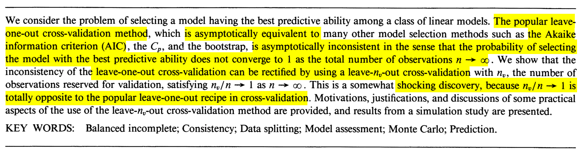
Figure 3.4: The abstract of Jun Shao’s Linear model selection by cross-validation (Shao 1993).

The Leave-One-Out Cross-Validation (LOOCV) error in a fitted linear model is defined as \[\begin{align} \mathrm{LOOCV}:=\frac{1}{n}\sum_{i=1}^n(Y_i-\hat{Y}_{i,-i})^2,\tag{3.3} \end{align}\] where $\hat{Y}_{i,-i}$ is the prediction of the $i$-th observation in a linear model that has been fitted without the $i$-th datum $(X_{i1},\ldots,X_{ip},Y_i).$ That is, $\hat{Y}_{i,-i}=\hat{\beta}_{0,-i}+\hat{\beta}_{1,-i}X_{i1}+\cdots+\hat{\beta}_{p,-i}X_{ip},$ where $\hat{\boldsymbol{\beta}}_{-i}$ are the estimated coefficients from the sample $\{(X_{j1},\ldots,X_{jp},Y_j)\}_{j=1,\, j\neq i}^n.$ Model selection based on LOOCV chooses the model with minimum error (3.3) within a list of candidate models. Note that the computation of $\mathrm{LOOCV}$ requires, in principle, to fit $n$ separate linear models, predict, and then aggregate. However, an algebraic shortcut based on (4.25) allows to compute (3.3) using a single linear fit.

We carry out a small simulation study in order to illustrate the consistency property (3.2) of BIC and the inconsistency of model selection by AIC and LOOCV. For that, we consider the linear model \[\begin{align} \begin{split} Y&=\beta_0+\beta_1X_1+\beta_2X_2+\beta_3X_3+\beta_4X_4+\beta_5X_5+\varepsilon,\\ \boldsymbol{\beta}&=(0.5,1,1,0,0,0)', \end{split} \tag{3.4} \end{align}\] where $X_j\sim\mathcal{N}(0,1)$ for $j=1,\ldots,5$ (independently) and $\varepsilon\sim\mathcal{N}(0,1).$ Only the first two predictors are relevant, the last three are “garbage” predictors. For a given sample, model selection is performed by selecting among the $2^5$ possible fitted models the ones with minimum AIC, BIC, and LOOCV. The experiment is repeated $M=500$ times for sample sizes $n=2^\ell,$ $\ell=3,\ldots,12,$ and the estimated probability of selecting the correct model (the one only involving $X_1$ and $X_2$) is displayed in Figure 3.5. The figure evidences empirically several interesting results:

LOOCV and AIC are asymptotically equivalent. For large $n,$ they tend to select the same model and hence their estimated probabilities of selecting the true model are almost equal. For small $n,$ there are significant differences between them.
The BIC is consistent in selecting the true model, and its probability of doing so quickly approaches $1,$ as anticipated by (3.2).
The AIC and LOOCV are inconsistent in selecting the true model. Despite the sample size $n$ doubling at each step, their probability of recovering the true model gets stuck at about $0.60.$
Even for moderate $n$’s, the probability of recovering the true model by BIC quickly outperforms those of AIC/LOOCV.

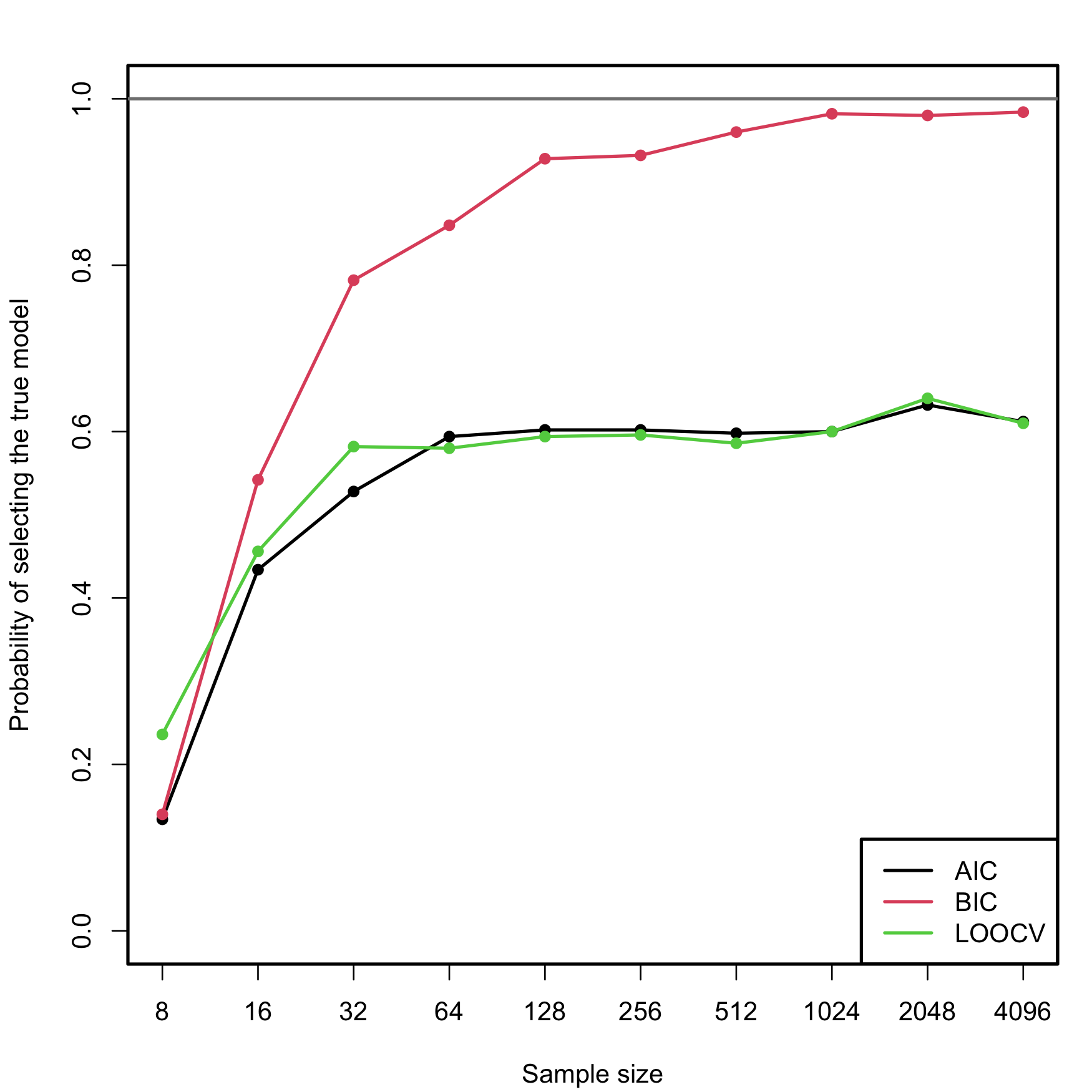
$Estimation of the probability of selecting the correct model by minimizing the AIC, BIC, and LOOCV criteria, done for an exhaustive search with $p=5$ predictors. The correct model contained two predictors. The probability was estimated with $M=500$ Monte Carlo runs. The horizontal axis is in logarithmic scale. The estimated proportion of true model recoveries with BIC for $n=4096$ is $0.984$.$

Figure 3.5: Estimation of the probability of selecting the correct model by minimizing the AIC, BIC, and LOOCV criteria, done for an exhaustive search with $p=5$ predictors. The correct model contained two predictors. The probability was estimated with $M=500$ Monte Carlo runs. The horizontal axis is in logarithmic scale. The estimated proportion of true model recoveries with BIC for $n=4096$ is $0.984$.

Implement the simulation study behind Figure 3.5:

Sample from (3.4), but take $p=4.$
Fit the $2^p$ possible models.
Select the best model according to the AIC and BIC.
Repeat Steps 1–3 $M=100$ times. Estimate by Monte Carlo the probability of selecting the true model.
Move $n$ in a range from $10$ to $200.$

Once you have a working solution, increase $(p, n, M)$ to approach the settings in Figure 3.5 (or go beyond!).

Modify the Step 3 of the previous exercise to:

Select the best model according to the $R^2_\text{Adj}$ and investigate its consistency in model selection.
Add the LOOCV criterion in order to fully replicate Figure 3.5. Hint: you may want to adapt (4.25) to your needs in order to reduce computation time.

Investigate what happens with the probability of selecting the true model using BIC and AIC if the exhaustive search is replaced by a stepwise selection. Precisely, do:

Sample from (3.4), but take $p=10$ (pad $\boldsymbol{\beta}$ with zeros).
Run a forward-backward stepwise search, both for the AIC and BIC.
Repeat Steps 1–2 $M=100$ times. Estimate by Monte Carlo the probability of selecting the true model.
Move $n$ in a range from $20$ to $200.$

Once you have a working solution, increase $(n, M)$ to approach the settings in Figure 3.5 (or go beyond!).

Shao (1993)’s modification on how to make consistent the model selection by cross-validation is shocking. As in LOOCV, one has to split the sample of size $n$ into two subsets: a training set, of size $n_t,$ and a validation set, of size $n_v.$ Of course, $n=n_t+n_v.$ However, totally opposite to LOOCV, where $n_t=n-1$ and $n_v=1,$ the modification required is to choose $n_v$ asymptotically equal to $n$, in the sense that $n_v/n\to1$ as $n\to\infty.$ An example would be to take $n_v=n-20$ and $n_t=20.$ But $n_v=n/2$ and $n_t=n/2,$ a typical choice, would not make the selection consistent! Shao (1993)’s result gives a great insight: the difficulty in model selection lies in the comparison of models, not in their estimation, and the sample information has to be disproportionately allocated to the comparison task to achieve a consistent model selection device.

Verify Shao (1993)’s result by constructing the analogous of Figure 3.5 for the following choices of $(n_t,n_v)$:

$n_t=n-1,$ $n_v=1$ (LOOCV).
$n_t=n/2,$ $n_v=n/2.$
$n_t=n/4,$ $n_v=(3/4)n.$
$n_t=5p,$ $n_v=n-5p.$

Use first $p=4$ predictors, $M=100$ Monte Carlo runs, and move $n$ in a range from $20$ to $200.$ Then increase the settings to approach those of Figure 3.5.

References

Schwarz, G. 1978. “Estimating the Dimension of a Model.” The Annals of Statistics 6 (2): 461–64. https://doi.org/10.1214/aos/1176344136.

Shao, J. 1993. “Linear Model Selection by Cross-Validation.” Journal of the American Statistical Association 88 (422): 486–94. https://doi.org/10.2307/2290328.

Applying its formula, we would obtain $\hat\sigma^2=0/0$ and so $\hat\sigma^2$ will not be defined.↩︎
Of course, with the same responses.↩︎
Recall that $\log(n)>2$ if $n\geq8.$↩︎
Also, because the BIC is consistent, see Section 3.2.2.↩︎
Since we have to take $p$ binary decisions on whether to include or not each of the $p$ predictors.↩︎
The function always prints ‘AIC’, even if ‘BIC’ is employed.↩︎
Note the - before FrancePop. Note also the convenient sorting of the BICs in an increasing form, so that the next best action always corresponds to the first row.↩︎
If possible!↩︎
The specifics of this result for the linear model are given in Schwarz (1978).↩︎
Cross-validation and its different variants are formally addressed at the end of Section 3.6.2.↩︎