3.6 Dimension reduction techniques

As we have seen in Section 3.2, the selection of the best linear model from a set of \(p\) predictors is a challenging task that increases with the dimension of the problem, that is, with \(p.\) In addition to the growth of the set of possible models as \(p\) grows, the model space becomes more complicated to explore due to the potential multicollinearity among the predictors. We will see in this section two methods to deal with these two problems simultaneously.

3.6.1 Review on principal component analysis

Principal Component Analysis (PCA) is a multivariate technique designed to summarize the most important features and relations of \(p\) numerical random variables \(X_1,\ldots,X_p.\) PCA computes a new set of variables, the principal components \(\Gamma_1,\ldots, \Gamma_p,\) that contain the same information as \(X_1,\ldots,X_p\) but expressed in a more convenient way. The goal of PCA is to retain only a limited number \(\ell,\) \(1\leq \ell\leq p,\) of principal components that explain most of the information, therefore performing dimension reduction.

If \(X_1,\ldots,X_p\) are centered⁸⁰, then the principal components are orthonormal linear combinations of \(X_1,\ldots,X_p\):

\[\begin{align} \Gamma_j:=a_{1j}X_1+a_{2j}X_2+\cdots+a_{pj}X_p=\mathbf{a}_j'\mathbf{X},\quad j=1,\ldots,p,\tag{3.9} \end{align}\]

where \(\mathbf{a}_j:=(a_{1j},\ldots,a_{pj})',\) \(\mathbf{X}:=(X_1,\ldots,X_p)',\) and the orthonormality condition is

\[\begin{align*} \mathbf{a}_i'\mathbf{a}_j=\begin{cases}1,&\text{if } i=j,\\0,&\text{if } i\neq j.\end{cases} \end{align*}\]

Remarkably, PCA computes the principal components in an ordered way: \(\Gamma_1\) is the principal component that explains the most of the information (quantified as the variance) of \(X_1,\ldots,X_p,\) and then the explained information decreases monotonically down to \(\Gamma_p,\) the principal component that explains the least information. Precisely:

\[\begin{align} \mathbb{V}\mathrm{ar}[\Gamma_1]\geq \mathbb{V}\mathrm{ar}[\Gamma_2]\geq\ldots\geq\mathbb{V}\mathrm{ar}[\Gamma_p].\tag{3.10} \end{align}\]

Mathematically, PCA computes the spectral decomposition⁸¹ of the covariance matrix \(\boldsymbol\Sigma:=\mathbb{V}\mathrm{ar}[\mathbf{X}]\):

\[\begin{align*} \boldsymbol\Sigma=\mathbf{A}\boldsymbol\Lambda\mathbf{A}', \end{align*}\]

where \(\boldsymbol\Lambda=\mathrm{diag}(\lambda_1,\ldots,\lambda_p)\) contains the eigenvalues of \(\boldsymbol\Sigma\) and \(\mathbf{A}\) is the orthogonal matrix⁸² whose columns are the unit-norm eigenvectors of \(\boldsymbol\Sigma.\) The matrix \(\mathbf{A}\) gives, thus, the coefficients of the orthonormal linear combinations:

\[\begin{align*} \mathbf{A}=\begin{pmatrix} \mathbf{a}_1 & \mathbf{a}_2 & \cdots & \mathbf{a}_p \end{pmatrix}=\begin{pmatrix} a_{11} & a_{12} & \cdots & a_{1p} \\ a_{21} & a_{22} & \cdots & a_{2p} \\ \vdots & \vdots & \ddots & \vdots \\ a_{p1} & a_{p2} & \cdots & a_{pp} \end{pmatrix}. \end{align*}\]

If the variables are not centered, the computation of the principal components is done by first subtracting \(\boldsymbol\mu=\mathbb{E}[\mathbf{X}]\) and then premultiplying with \(\mathbf{A}'\):

\[\begin{align} \boldsymbol{\Gamma}=\mathbf{A}'(\mathbf{X}-\boldsymbol{\mu}),\tag{3.11} \end{align}\]

where \(\boldsymbol{\Gamma}=(\Gamma_1,\ldots,\Gamma_p)',\) \(\mathbf{X}=(X_1,\ldots,X_p)',\) and \(\boldsymbol{\mu}=(\mu_1,\ldots,\mu_p)'.\) Note that, because of (1.3) and (3.11),

\[\begin{align} \mathbb{V}\mathrm{ar}[\boldsymbol{\Gamma}]=\mathbf{A}'\boldsymbol{\Sigma}\mathbf{A}=\mathbf{A}'\mathbf{A}\boldsymbol{\Lambda}\mathbf{A}'\mathbf{A}=\boldsymbol{\Lambda}. \end{align}\]

Therefore, \(\mathbb{V}\mathrm{ar}[\Gamma_j]=\lambda_j,\) \(j=1,\ldots,p,\) and as a consequence (3.10) indeed holds.

Also, from (3.11), it is evident that we can express the random vector \(\mathbf{X}\) in terms of \(\boldsymbol{\Gamma}\):

\[\begin{align} \mathbf{X}=\boldsymbol{\mu}+\mathbf{A}\boldsymbol{\Gamma},\tag{3.12} \end{align}\]

which admits an insightful interpretation: \(\boldsymbol{\Gamma}\) is an uncorrelated⁸³ vector that, once rotated by \(\mathbf{A}\) and translated to the location \(\boldsymbol{\mu},\) produces exactly \(\mathbf{X}.\) Therefore, \(\boldsymbol{\Gamma}\) contains the same information as \(\mathbf{X}\) but rearranged in a more convenient way, because the principal components are centered and uncorrelated between them:

\[\begin{align*} \mathbb{E}[\Gamma_i]=0\text{ and }\mathrm{Cov}[\Gamma_i,\Gamma_j]=\begin{cases}\lambda_i,&\text{if } i=j,\\0,&\text{if } i\neq j.\end{cases} \end{align*}\]

Due to the uncorrelation of \(\boldsymbol{\Gamma},\) we can measure the total variance of \(\boldsymbol{\Gamma}\) as \(\sum_{j=1}^p\mathbb{V}\mathrm{ar}[\Gamma_j]=\sum_{j=1}^p\lambda_j.\) Consequently, we can define the proportion of variance explained by the first \(\ell\) principal components, \(1\leq \ell\leq p,\) as

\[\begin{align*} \frac{\sum_{j=1}^\ell\lambda_j}{\sum_{j=1}^p\lambda_j}. \end{align*}\]

In the sample case⁸⁴ where a sample \(\mathbf{X}_1,\ldots,\mathbf{X}_n\) is given and \(\boldsymbol\mu\) and \(\boldsymbol\Sigma\) are unknown, \(\boldsymbol\mu\) is replaced by the sample mean \(\bar{\mathbf{X}}\) and \(\boldsymbol\Sigma\) by the sample variance-covariance matrix \(\mathbf{S}=\frac{1}{n}\sum_{i=1}^n(\mathbf{X}_i-\bar{\mathbf{X}})(\mathbf{X}_i-\bar{\mathbf{X}})'.\) Then, the spectral decomposition of \(\mathbf{S}\) is computed⁸⁵. This gives \(\hat{\mathbf{A}},\) the matrix of loadings, and produces the scores of the data:

\[\begin{align*} \hat{\boldsymbol{\Gamma}}_1:=\hat{\mathbf{A}}'(\mathbf{X}_1-\bar{\mathbf{X}}),\ldots,\hat{\boldsymbol{\Gamma}}_n:=\hat{\mathbf{A}}'(\mathbf{X}_n-\bar{\mathbf{X}}). \end{align*}\]

The scores are centered, uncorrelated, and have sample variances in each vector’s entry that are sorted in a decreasing way. The scores are the data coordinates with respect to the principal component basis.

The maximum number of principal components that can be determined from a sample \(\mathbf{X}_1,\ldots,\mathbf{X}_n\) is \(\min(n-1,p),\) assuming that the matrix formed by \(\left(\mathbf{X}_1 \cdots \mathbf{X}_n\right)\) is of full rank (i.e., if the rank is \(\min(n,p)\)). If \(n\geq p\) and the variables \(X_1,\ldots,X_p\) are such that only \(r\) of them are linearly independent, then the maximum is \(\min(n-1,r).\)

Let’s see an example of these concepts in La Liga 2015/2016 dataset. It contains the standings and team statistics for La Liga 2015/2016.

laliga <- readxl::read_excel("la-liga-2015-2016.xlsx", sheet = 1, col_names = TRUE)
laliga <- as.data.frame(laliga) # Avoid tibble since it drops row.names

A quick preprocessing gives:

rownames(laliga) <- laliga$Team # Set teams as case names to avoid factors
laliga$Team <- NULL
laliga <- laliga[, -c(2, 8)] # Do not add irrelevant information
summary(laliga)
##      Points           Wins           Draws           Loses        Goals.scored    Goals.conceded 
##  Min.   :32.00   Min.   : 8.00   Min.   : 4.00   Min.   : 4.00   Min.   : 34.00   Min.   :18.00  
##  1st Qu.:41.25   1st Qu.:10.00   1st Qu.: 8.00   1st Qu.:12.00   1st Qu.: 40.00   1st Qu.:42.50  
##  Median :44.50   Median :12.00   Median : 9.00   Median :15.50   Median : 45.50   Median :52.50  
##  Mean   :52.40   Mean   :14.40   Mean   : 9.20   Mean   :14.40   Mean   : 52.15   Mean   :52.15  
##  3rd Qu.:60.50   3rd Qu.:17.25   3rd Qu.:10.25   3rd Qu.:18.25   3rd Qu.: 51.25   3rd Qu.:63.25  
##  Max.   :91.00   Max.   :29.00   Max.   :18.00   Max.   :22.00   Max.   :112.00   Max.   :74.00  
##  Percentage.scored.goals Percentage.conceded.goals     Shots       Shots.on.goal   Penalties.scored  Assistances   
##  Min.   :0.890           Min.   :0.470             Min.   :346.0   Min.   :129.0   Min.   : 1.00    Min.   :23.00  
##  1st Qu.:1.050           1st Qu.:1.115             1st Qu.:413.8   1st Qu.:151.2   1st Qu.: 1.00    1st Qu.:28.50  
##  Median :1.195           Median :1.380             Median :438.0   Median :165.0   Median : 3.00    Median :32.50  
##  Mean   :1.371           Mean   :1.371             Mean   :452.4   Mean   :173.1   Mean   : 3.45    Mean   :37.85  
##  3rd Qu.:1.347           3rd Qu.:1.663             3rd Qu.:455.5   3rd Qu.:180.0   3rd Qu.: 4.50    3rd Qu.:36.75  
##  Max.   :2.950           Max.   :1.950             Max.   :712.0   Max.   :299.0   Max.   :11.00    Max.   :90.00  
##    Fouls.made    Matches.without.conceding  Yellow.cards     Red.cards       Offsides     
##  Min.   :385.0   Min.   : 4.0              Min.   : 66.0   Min.   :1.00   Min.   : 72.00  
##  1st Qu.:483.8   1st Qu.: 7.0              1st Qu.: 97.0   1st Qu.:4.00   1st Qu.: 83.25  
##  Median :530.5   Median :10.5              Median :108.5   Median :5.00   Median : 88.00  
##  Mean   :517.6   Mean   :10.7              Mean   :106.2   Mean   :5.05   Mean   : 92.60  
##  3rd Qu.:552.8   3rd Qu.:13.0              3rd Qu.:115.2   3rd Qu.:6.00   3rd Qu.:103.75  
##  Max.   :654.0   Max.   :24.0              Max.   :141.0   Max.   :9.00   Max.   :123.00

Let’s check that R’s function for PCA, princomp, returns the same principal components we outlined in the theory.

# PCA
pcaLaliga <- princomp(laliga, fix_sign = TRUE)
summary(pcaLaliga)
## Importance of components:
##                             Comp.1     Comp.2      Comp.3      Comp.4      Comp.5     Comp.6      Comp.7      Comp.8
## Standard deviation     104.7782561 48.5461449 22.13337511 12.66692413 8.234215354 7.83426116 6.068864168 4.137079559
## Proportion of Variance   0.7743008  0.1662175  0.03455116  0.01131644 0.004782025 0.00432876 0.002597659 0.001207133
## Cumulative Proportion    0.7743008  0.9405183  0.97506949  0.98638593 0.991167955 0.99549671 0.998094374 0.999301507
##                              Comp.9      Comp.10      Comp.11      Comp.12      Comp.13      Comp.14      Comp.15
## Standard deviation     2.0112480391 1.8580509157 1.126111e+00 9.568824e-01 4.716064e-01 1.707105e-03 8.365534e-04
## Proportion of Variance 0.0002852979 0.0002434908 8.943961e-05 6.457799e-05 1.568652e-05 2.055361e-10 4.935768e-11
## Cumulative Proportion  0.9995868048 0.9998302956 9.999197e-01 9.999843e-01 1.000000e+00 1.000000e+00 1.000000e+00
##                        Comp.16 Comp.17
## Standard deviation           0       0
## Proportion of Variance       0       0
## Cumulative Proportion        1       1
# The standard deviations are the square roots of the eigenvalues
# The cumulative proportion of variance explained accumulates the
# variance explained starting at the first component

# We use fix_sign = TRUE so that the signs of the loadings are
# determined by the first element of each loading, set to be
# non-negative. Otherwise, the signs could change for different OS /
# R versions yielding to opposite interpretations of the PCs

# Plot of variances of each component (screeplot)
plot(pcaLaliga, type = "l")

# Useful for detecting an "elbow" in the graph whose location gives the
# "right" number of components to retain. Ideally, this elbow appears
# when the next variances are almost similar and notably smaller when
# compared with the previous

# Alternatively: plot of the cumulated percentage of variance
# barplot(cumsum(pcaLaliga$sdev^2) / sum(pcaLaliga$sdev^2))

# Computation of PCA from the spectral decomposition
n <- nrow(laliga)
eig <- eigen(cov(laliga) * (n - 1) / n) # By default, cov() computes the
# quasi-variance-covariance matrix that divides by n - 1, but PCA and princomp
# consider the sample variance-covariance matrix that divides by n
A <- eig$vectors

# Same eigenvalues
pcaLaliga$sdev^2 - eig$values
##        Comp.1        Comp.2        Comp.3        Comp.4        Comp.5        Comp.6        Comp.7        Comp.8 
## -5.456968e-12 -1.364242e-12  0.000000e+00 -4.263256e-13 -2.415845e-13 -1.278977e-13 -3.552714e-14 -4.263256e-14 
##        Comp.9       Comp.10       Comp.11       Comp.12       Comp.13       Comp.14       Comp.15       Comp.16 
## -2.025047e-13 -7.549517e-14 -1.088019e-14 -3.108624e-15 -1.626477e-14 -3.685726e-15  1.036604e-15 -2.025796e-13 
##       Comp.17 
##  1.435137e-12

# The eigenvectors (the a_j vectors) are the column vectors in $loadings
pcaLaliga$loadings
## 
## Loadings:
##                           Comp.1 Comp.2 Comp.3 Comp.4 Comp.5 Comp.6 Comp.7 Comp.8 Comp.9 Comp.10 Comp.11 Comp.12
## Points                     0.125         0.497  0.195  0.139  0.340         0.425         0.379   0.129   0.166 
## Wins                                     0.184                0.175         0.134 -0.198                  0.139 
## Draws                                                  0.101 -0.186                0.608  0.175   0.185  -0.251 
## Loses                                   -0.129        -0.114               -0.157 -0.410 -0.243  -0.166   0.112 
## Goals.scored               0.181         0.251 -0.186 -0.169  0.399  0.335 -0.603 -0.155  0.129   0.289  -0.230 
## Goals.conceded                          -0.471 -0.493 -0.277  0.257  0.280  0.441 -0.118  0.297                 
## Percentage.scored.goals                                                                                         
## Percentage.conceded.goals                                                                                       
## Shots                      0.718  0.442 -0.342  0.255  0.241         0.188                                      
## Shots.on.goal              0.386  0.213  0.182 -0.287 -0.532 -0.163 -0.599                                      
## Penalties.scored                                                           -0.350  0.258  0.378  -0.661   0.456 
## Assistances                0.148         0.198        -0.173  0.362  0.216  0.215  0.356 -0.685  -0.265         
## Fouls.made                -0.480  0.844  0.166               -0.110                                             
## Matches.without.conceding                0.151  0.129               -0.182  0.176 -0.369         -0.376  -0.411 
## Yellow.cards              -0.141  0.144 -0.363  0.113  0.225  0.637 -0.550 -0.126  0.156                        
## Red.cards                                                                         -0.123 -0.157   0.405   0.666 
## Offsides                          0.108  0.202 -0.696  0.647        -0.106                                      
##                           Comp.13 Comp.14 Comp.15 Comp.16 Comp.17
## Points                     0.138                   0.240   0.345 
## Wins                       0.147                          -0.904 
## Draws                     -0.304                   0.554  -0.215 
## Loses                      0.156                   0.794   0.130 
## Goals.scored              -0.153                                 
## Goals.conceded                                                   
## Percentage.scored.goals           -0.760  -0.650                 
## Percentage.conceded.goals          0.650  -0.760                 
## Shots                                                            
## Shots.on.goal                                                    
## Penalties.scored          -0.114                                 
## Assistances               -0.102                                 
## Fouls.made                                                       
## Matches.without.conceding -0.664                                 
## Yellow.cards                                                     
## Red.cards                 -0.587                                 
## Offsides                                                         
## 
##                Comp.1 Comp.2 Comp.3 Comp.4 Comp.5 Comp.6 Comp.7 Comp.8 Comp.9 Comp.10 Comp.11 Comp.12 Comp.13 Comp.14
## SS loadings     1.000  1.000  1.000  1.000  1.000  1.000  1.000  1.000  1.000   1.000   1.000   1.000   1.000   1.000
## Proportion Var  0.059  0.059  0.059  0.059  0.059  0.059  0.059  0.059  0.059   0.059   0.059   0.059   0.059   0.059
## Cumulative Var  0.059  0.118  0.176  0.235  0.294  0.353  0.412  0.471  0.529   0.588   0.647   0.706   0.765   0.824
##                Comp.15 Comp.16 Comp.17
## SS loadings      1.000   1.000   1.000
## Proportion Var   0.059   0.059   0.059
## Cumulative Var   0.882   0.941   1.000

# The scores is the representation of the data in the principal components -
# it has the same information as laliga
head(round(pcaLaliga$scores, 4))
##                   Comp.1   Comp.2  Comp.3   Comp.4  Comp.5  Comp.6  Comp.7  Comp.8  Comp.9 Comp.10 Comp.11 Comp.12
## Barcelona       242.2392 -21.5810 25.3801 -17.4375 -7.1797  9.0814 -5.5920 -7.3615 -0.3716  1.7161  0.0265 -1.0948
## Real Madrid     313.6026  63.2024 -8.7570   8.5558  0.7119  0.2221  6.7035  2.4456  1.8388 -2.9661 -0.1345  0.3410
## Atlético Madrid  45.9939  -0.6466 38.5410  31.3888  3.9163  3.2904  0.2432  5.0913 -3.0444  2.0975  0.6771 -0.3986
## Villarreal      -96.2201 -42.9329 50.0036 -11.2420 10.4733  2.4294 -3.0183  0.1958  1.2106 -1.7453  0.1351 -0.5735
## Athletic         14.5173 -16.1897 18.8840  -0.4122 -5.6491 -6.9330  8.0653  2.4783 -2.6921  0.8950  0.1542  1.4715
## Celta           -13.0748   6.7925  5.2271  -9.0945  6.1265 11.8795 -2.6148  6.9707  3.0826  0.3130  0.0860  1.9159
##                 Comp.13 Comp.14 Comp.15 Comp.16 Comp.17
## Barcelona        0.1516 -0.0010  -2e-04       0       0
## Real Madrid     -0.0332  0.0015   4e-04       0       0
## Atlético Madrid -0.1809  0.0005  -1e-04       0       0
## Villarreal      -0.5894 -0.0001  -2e-04       0       0
## Athletic         0.1109 -0.0031  -3e-04       0       0
## Celta            0.3722 -0.0018   3e-04       0       0

# Uncorrelated
corrplot::corrplot(cor(pcaLaliga$scores), addCoef.col = "gray")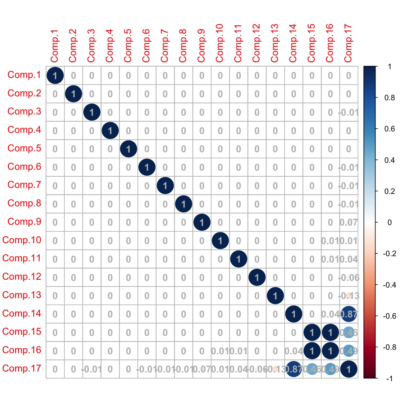

# Caution! What happened in the last columns? What happened is that the
# variance for the last principal components is close to zero (because there
# are linear dependencies on the variables; e.g., Points, Wins, Loses, Draws),
# so the computation of the correlation matrix becomes unstable for those
# variables (a 0/0 division takes place)

# Better to inspect the covariance matrix
corrplot::corrplot(cov(pcaLaliga$scores), addCoef.col = "gray", is.corr = FALSE)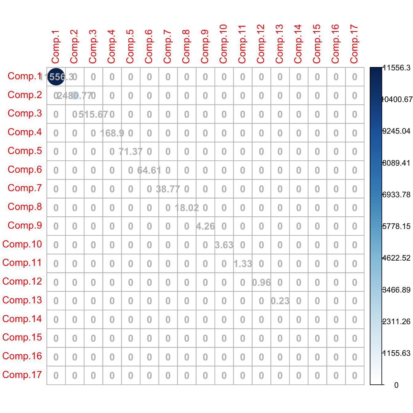

# The scores are A' * (X_i - mu). We center the data with scale()
# and then multiply each row by A'
scores <- scale(laliga, center = TRUE, scale = FALSE) %*% A

# Same as (but this is much slower)
# scores <- t(apply(scale(laliga, center = TRUE, scale = FALSE), 1,
#                   function(x) t(A) %*% x))

# Same scores (up to possible changes in signs)
max(abs(abs(pcaLaliga$scores) - abs(scores)))
## [1] 2.278507e-11

# Reconstruct the data from all the principal components
head(
  sweep(pcaLaliga$scores %*% t(pcaLaliga$loadings), 2, pcaLaliga$center, "+")
  )
##                 Points Wins Draws Loses Goals.scored Goals.conceded Percentage.scored.goals Percentage.conceded.goals
## Barcelona           91   29     4     5          112             29                    2.95                      0.76
## Real Madrid         90   28     6     4          110             34                    2.89                      0.89
## Atlético Madrid     88   28     4     6           63             18                    1.66                      0.47
## Villarreal          64   18    10    10           44             35                    1.16                      0.92
## Athletic            62   18     8    12           58             45                    1.53                      1.18
## Celta               60   17     9    12           51             59                    1.34                      1.55
##                 Shots Shots.on.goal Penalties.scored Assistances Fouls.made Matches.without.conceding Yellow.cards
## Barcelona         600           277               11          79        385                        18           66
## Real Madrid       712           299                6          90        420                        14           72
## Atlético Madrid   481           186                1          49        503                        24           91
## Villarreal        346           135                3          32        534                        17          100
## Athletic          450           178                3          42        502                        13           84
## Celta             442           170                4          43        528                        10          116
##                 Red.cards Offsides
## Barcelona               1      120
## Real Madrid             5      114
## Atlético Madrid         3       84
## Villarreal              4      106
## Athletic                5       92
## Celta                   6      103

An important issue when doing PCA is the scale of the variables, since the variance depends on the units in which the variable is measured⁸⁶. Therefore, when variables with different ranges are mixed, the variability of one may dominate the other merely due to a scale artifact. To prevent this, we standardize the dataset prior to do a PCA.

# Use cor = TRUE to standardize variables (all have unit variance)
# and avoid scale distortions
pcaLaligaStd <- princomp(x = laliga, cor = TRUE, fix_sign = TRUE)
summary(pcaLaligaStd)
## Importance of components:
##                           Comp.1    Comp.2     Comp.3     Comp.4     Comp.5     Comp.6     Comp.7      Comp.8
## Standard deviation     3.2918365 1.5511043 1.13992451 0.91454883 0.85765282 0.59351138 0.45780827 0.370649324
## Proportion of Variance 0.6374228 0.1415250 0.07643694 0.04919997 0.04326873 0.02072093 0.01232873 0.008081231
## Cumulative Proportion  0.6374228 0.7789478 0.85538472 0.90458469 0.94785342 0.96857434 0.98090308 0.988984306
##                             Comp.9     Comp.10     Comp.11      Comp.12     Comp.13      Comp.14      Comp.15
## Standard deviation     0.327182806 0.217470830 0.128381750 0.0976778705 0.083027923 2.582795e-03 1.226924e-03
## Proportion of Variance 0.006296976 0.002781974 0.000969522 0.0005612333 0.000405508 3.924019e-07 8.854961e-08
## Cumulative Proportion  0.995281282 0.998063256 0.999032778 0.9995940111 0.999999519 9.999999e-01 1.000000e+00
##                             Comp.16 Comp.17
## Standard deviation     9.256461e-09       0
## Proportion of Variance 5.040122e-18       0
## Cumulative Proportion  1.000000e+00       1

# The effects of the distortion can be clearly seen with the biplot
# Variability absorbed by Shots, Shots.on.goal, Fouls.made
biplot(pcaLaliga, cex = 0.75)

# The effects of the variables are more balanced
biplot(pcaLaligaStd, cex = 0.75)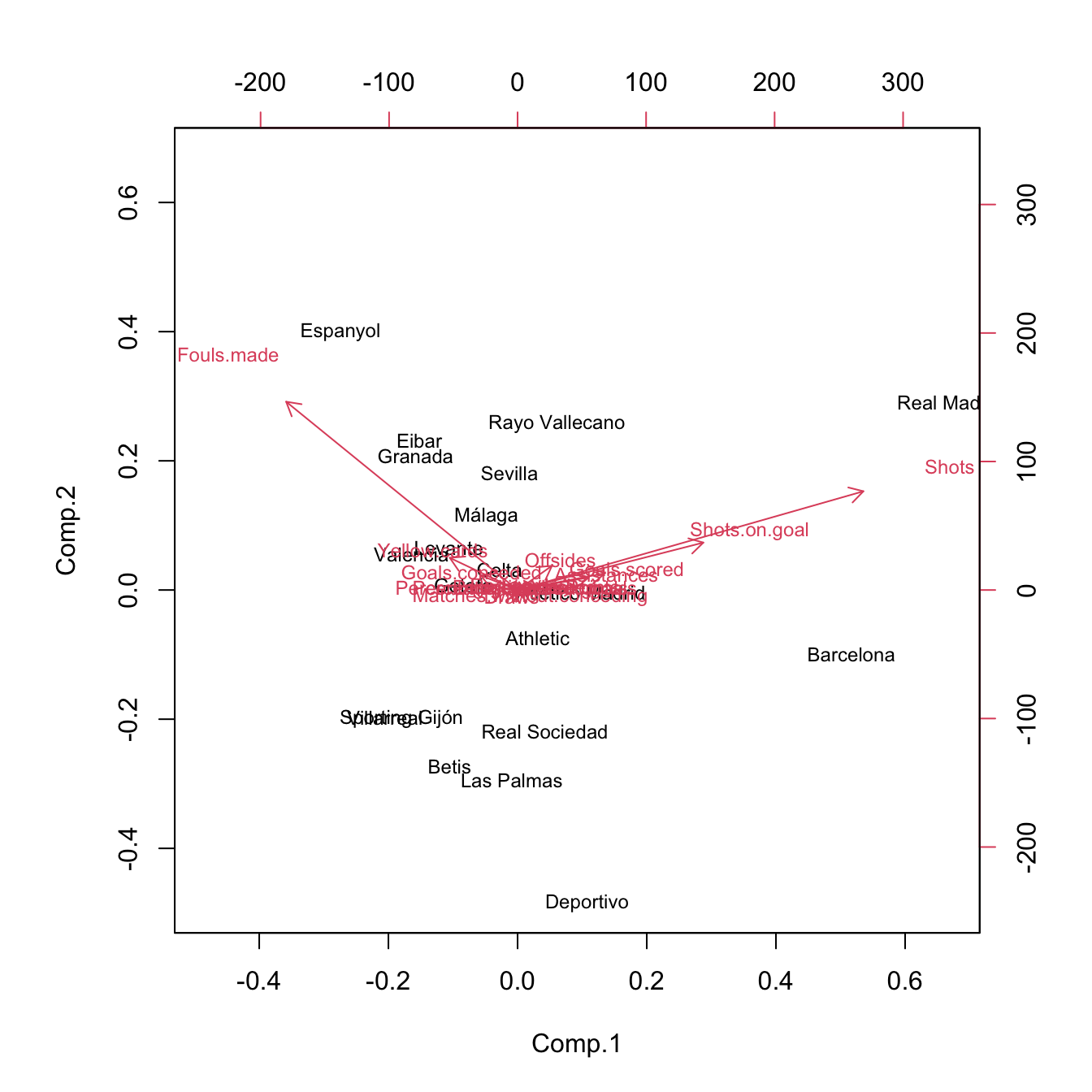

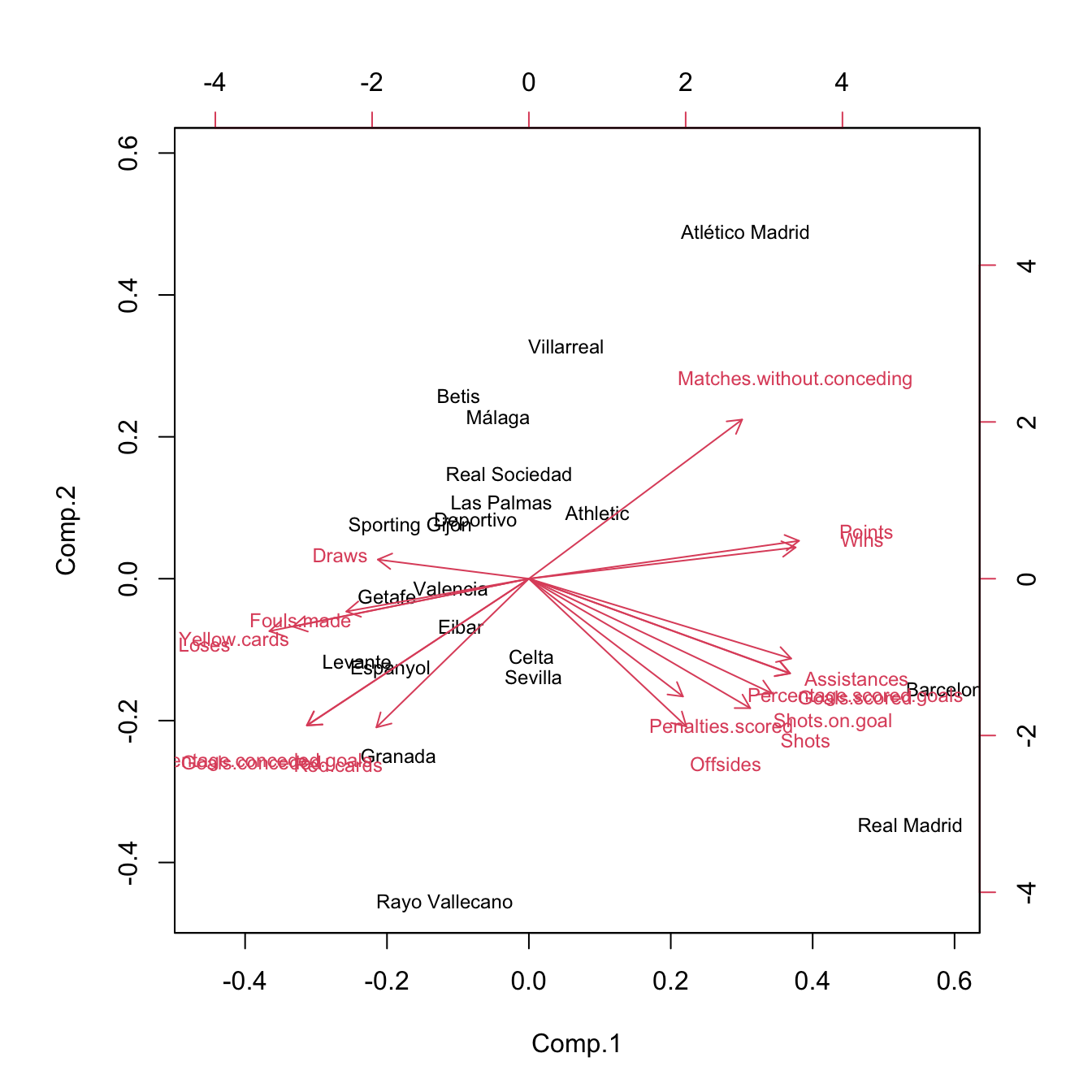
Figure 3.32: Biplots for laliga dataset, with unstandardized and standardized data, respectively.

The biplot⁸⁷ provides a powerful and succinct way of displaying the relevant information contained in the first two principal components. It shows:

1. The scores \(\{(\hat{\Gamma}_{i1},\hat{\Gamma}_{i2})\}_{i=1}^n\) by points (with optional text labels, depending if there are case names). These are the representations of the data in the first two principal components.
2. The loadings \(\{(\hat{a}_{j1},\hat{a}_{j2})\}_{j=1}^p\) by the arrows, centered at \((0,0).\) These are the representations of the variables in the first two principal components.

Let’s examine the population⁸⁸ arrow associated to the variable \(X_j.\) \(X_j\) is expressed in terms of \(\Gamma_1\) and \(\Gamma_2\) by the loadings \(a_{j1}\) and \(a_{j2}\;\)⁸⁹:

\[\begin{align*} X_j=a_{j1}\Gamma_{1} + a_{j2}\Gamma_{2} + \cdots + a_{jp}\Gamma_{p}\approx a_{j1}\Gamma_{1} + a_{j2}\Gamma_{2}. \end{align*}\]

The weights \(a_{j1}\) and \(a_{j2}\) have the same sign as \(\mathrm{Cor}(X_j,\Gamma_{1})\) and \(\mathrm{Cor}(X_j,\Gamma_{2}),\) respectively. The arrow associated to \(X_j\) is given by the segment joining \((0,0)\) and \((a_{j1},a_{j2}).\) Therefore:

• If the arrow points right (\(a_{j1}>0\)), there is positive correlation between \(X_j\) and \(\Gamma_1.\) Analogous if the arrow points left.
• If the arrow is approximately vertical (\(a_{j1}\approx0\)), there is uncorrelation between \(X_j\) and \(\Gamma_1.\)

Analogously:

• If the arrow points up (\(a_{j2}>0\)), there is positive correlation between \(X_j\) and \(\Gamma_2.\) Analogous if the arrow points down.
• If the arrow is approximately horizontal (\(a_{j2}\approx0\)), there is uncorrelation between \(X_j\) and \(\Gamma_2.\)

In addition, the magnitude of the arrow informs us about the strength of the correlation of \(X_j\) with \((\Gamma_{1}, \Gamma_{2}).\)

The biplot also informs about the direct relation between variables, at sight of their expressions in \(\Gamma_1\) and \(\Gamma_2.\) The angle of the arrows of variable \(X_j\) and \(X_k\) gives an approximation to the correlation between them, \(\mathrm{Cor}(X_j,X_k)\):

• If \(\text{angle}\approx 0^\circ,\) the two variables are highly positively correlated.
• If \(\text{angle}\approx 90^\circ,\) they are approximately uncorrelated.
• If \(\text{angle}\approx 180^\circ,\) the two variables are highly negatively correlated.

The insights obtained from the approximate correlations between variables are as precise as the percentage of variance explained by the first two principal components.

Figure 3.33: Biplot for laliga dataset. The interpretations of the first two principal components are driven by the signs of the variables inside them (directions of the arrows) and by the strength of their correlations with the variables (length of the arrows). The scores of the data serve also to cluster similar observations according to their proximity in the biplot.

Some interesting insights in La Liga 2015/2016 biplot, obtained from the previous remarks, are⁹⁰:

• The first component can be regarded as the performance of a team during the season. It is positively correlated with Wins, Points, etc. and negatively correlated with Draws, Loses, Yellow.cards, etc. The best performing teams are not surprising: Barcelona, Real Madrid, and Atlético Madrid. On the other hand, among the worst-performing teams are Levante, Getafe, and Granada.
• The second component can be seen as the efficiency of a team (obtaining points with little participation in the game). Using this interpretation we can see that Atlético Madrid and Villareal were the most efficient teams and that Rayo Vallecano and Real Madrid were the most inefficient.
• Offsides is approximately uncorrelated with Red.cards and Matches.without.conceding.

A 3D representation of the biplot can be computed through:

pca3d::pca3d(pcaLaligaStd, show.labels = TRUE, biplot = TRUE)
## [1] 0.1747106 0.0678678 0.0799681
rgl::rglwidget()

Finally, the biplot function allows to construct the biplot using two arbitrary principal components using the choices argument. Keep in mind than these pseudo-biplots will explain a lower proportion of variance than the default choices = 1:2:

biplot(pcaLaligaStd, choices = c(1, 3)) # 0.7138 proportion of variance
biplot(pcaLaligaStd, choices = c(2, 3)) # 0.2180 proportion of variance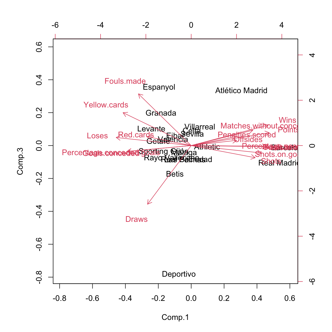

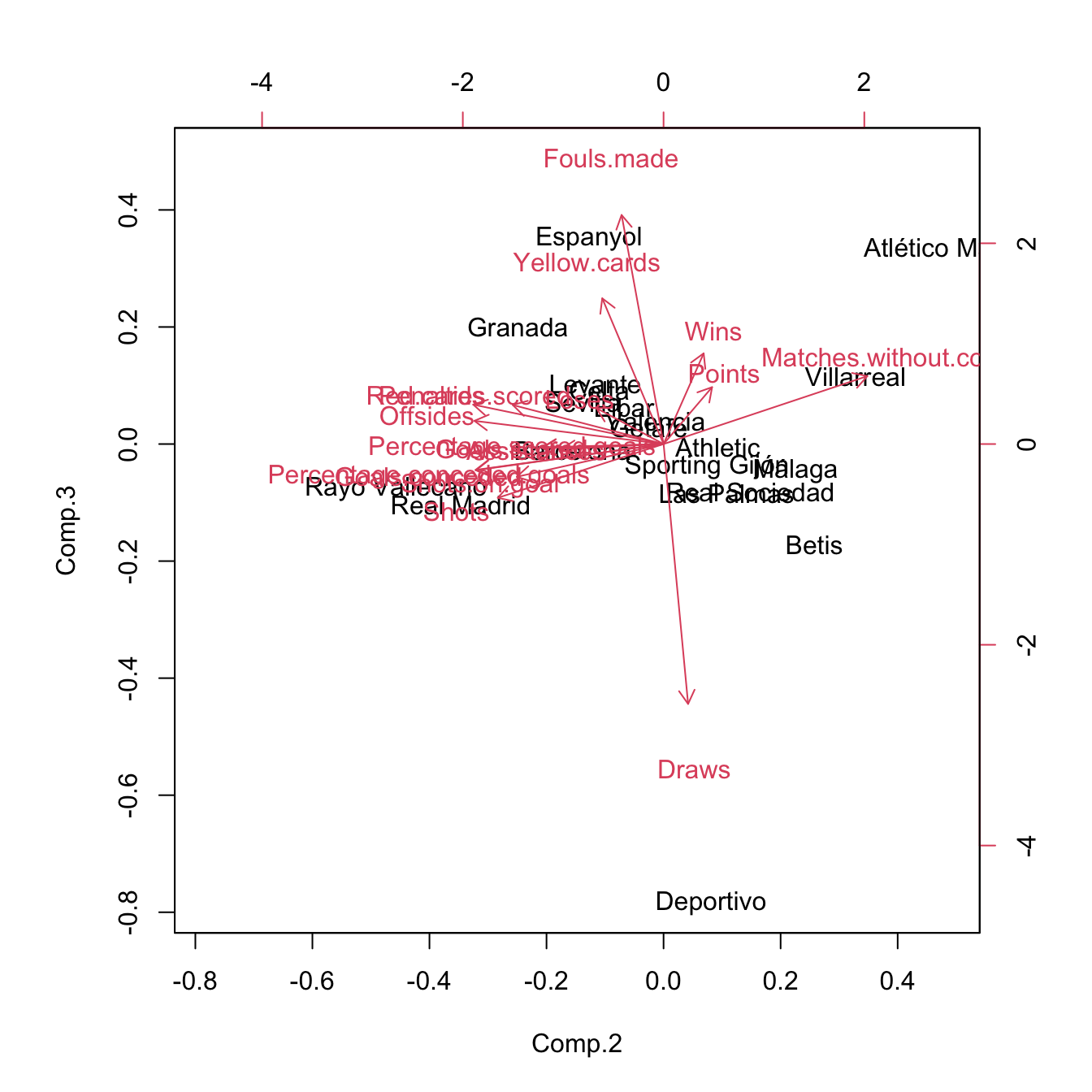
Figure 3.34: Pseudo-biplots for laliga dataset based on principal components 1 and 3, and principal components 2 and 3, respectively.

At the sight of the previous plots, can you think about an interpretation for the third principal component?

3.6.2 Principal components regression

The key idea behind Principal Components Regression (PCR) is to regress the response \(Y\) in a set of principal components \(\Gamma_1,\ldots,\Gamma_\ell\) obtained from the predictors \(X_1,\ldots,X_p,\) where \(\ell<p.\) The motivation is that often a small number of principal components is enough to explain most of the variability of the predictors and consequently their relationship with \(Y\;\)⁹¹. Therefore, we look for fitting the linear model⁹²

\[\begin{align} Y=\alpha_0+\alpha_1\Gamma_1+\cdots+\alpha_\ell\Gamma_\ell+\varepsilon.\tag{3.13} \end{align}\]

The main advantages of PCR are two:

1. Multicollinearity is avoided by design: \(\Gamma_1,\ldots,\Gamma_\ell\) are uncorrelated between them.
2. There are less coefficients to estimate (\(\ell\) instead of \(p\)), hence the accuracy of the estimation increases.

However, keep in mind that PCR affects the linear model in two fundamental ways:

1. Interpretation of the coefficients is not directly related with the predictors, but with the principal components. Hence, the interpretability of a given coefficient in the regression model is tied to the interpretability of the associated principal component.
2. Prediction needs an extra step, since it is required to obtain the scores of the new observations of the predictors.

The first point is elaborated next. The PCR model (3.13) can be seen as a linear model expressed in terms of the original predictors. To make this point clearer, let’s re-express (3.13) as

\[\begin{align} Y=\alpha_0+\boldsymbol{\Gamma}_{1:\ell}'\boldsymbol{\alpha}_{1:\ell}+\varepsilon,\tag{3.14} \end{align}\]

where the subindex \(1:\ell\) denotes the inclusion of the vector entries from \(1\) to \(\ell.\) Now, we can express the PCR problem (3.14) in terms of the original predictors⁹³:

\[\begin{align*} Y&=\alpha_0+(\mathbf{A}_{1:\ell}'(\mathbf{X}-\boldsymbol{\mu}))'\boldsymbol{\alpha}_{1:\ell}+\varepsilon\\ &=(\alpha_0-\boldsymbol{\mu}'\mathbf{A}_{1:\ell}\boldsymbol{\alpha}_{1:\ell})+\mathbf{X}'\mathbf{A}_{1:\ell}\boldsymbol{\alpha}_{1:\ell}+\varepsilon\\ &=\gamma_0+\mathbf{X}'\boldsymbol{\gamma}_{1:p}+\varepsilon, \end{align*}\]

where \(\mathbf{A}_{1:\ell}\) represents the \(\mathbf{A}\) matrix with only its first \(\ell\) columns and

\[\begin{align} \gamma_0:=\alpha_0-\boldsymbol{\mu}'\mathbf{A}_{1:\ell}\boldsymbol{\alpha}_{1:\ell},\quad \boldsymbol{\gamma}_{1:p}:=\mathbf{A}_{1:\ell}\boldsymbol{\alpha}_{1:\ell}.\tag{3.15} \end{align}\]

In other words, the coefficients \(\boldsymbol{\alpha}_{1:\ell}\) of the PCR done with \(\ell\) principal components in (3.13) translate into the coefficients (3.15) of the linear model based on the \(p\) original predictors:

\[\begin{align*} Y=\gamma_0+\gamma_1X_1+\cdots+\gamma_pX_p+\varepsilon. \end{align*}\]

In the sample case, we have that

\[\begin{align} \hat{\gamma}_0=\hat\alpha_0-\bar{\mathbf{X}}'\hat{\mathbf{A}}_{1:\ell}\hat{\boldsymbol{\alpha}}_{1:\ell},\quad \hat{\boldsymbol{\gamma}}_{1:p}=\hat{\mathbf{A}}_{1:\ell}\hat{\boldsymbol{\alpha}}_{1:\ell}.\tag{3.16} \end{align}\]

Notice that \(\hat{\boldsymbol{\gamma}}\) is not the least squares estimator performed with the original predictors, that we use to denote by \(\hat{\boldsymbol{\beta}}.\) \(\hat{\boldsymbol{\gamma}}\) contains the coefficients of the PCR that are associated to the original predictors. Consequently, \(\hat{\boldsymbol{\gamma}}\) is useful for the interpretation of the linear model produced by PCR, as it can be interpreted in the same way \(\hat{\boldsymbol{\beta}}\) was⁹⁴.

Finally, remember that the usefulness of PCR relies on how well we are able to reduce the dimensionality⁹⁵ of the predictors and the veracity of the assumption that the \(\ell\) principal components are related with \(Y.\)

Keep in mind that PCR considers the PCA done in the set of predictors, this is, we exclude the response for obvious reasons (a perfect and useless fit). It is important to remove the response from the call to princomp if we want to use the output in lm.

We see now two approaches for performing PCR, which we illustrate with the laliga dataset. The common objective is to predict Points using the remaining variables (excluding those directly related: Wins, Draws, Loses, and Matches.without.conceding) in order to quantify, explain, and predict the final points of a team from its performance.

The first approach combines the use of the princomp and lm functions. Its strong points are that is both able to predict and explain, and is linked with techniques we have employed so far. The weak point is that it requires extra coding.

# A linear model is problematic
mod <- lm(Points ~ . - Wins - Draws - Loses - Matches.without.conceding,
          data = laliga)
summary(mod) # Lots of non-significant predictors
## 
## Call:
## lm(formula = Points ~ . - Wins - Draws - Loses - Matches.without.conceding, 
##     data = laliga)
## 
## Residuals:
##     Min      1Q  Median      3Q     Max 
## -5.2117 -1.4766  0.0544  1.9515  4.1422 
## 
## Coefficients:
##                             Estimate Std. Error t value Pr(>|t|)  
## (Intercept)                 77.11798   26.12915   2.951   0.0214 *
## Goals.scored               -28.21714   17.44577  -1.617   0.1498  
## Goals.conceded             -24.23628   15.45595  -1.568   0.1608  
## Percentage.scored.goals   1066.98731  655.69726   1.627   0.1477  
## Percentage.conceded.goals  896.94781  584.97833   1.533   0.1691  
## Shots                       -0.10246    0.07754  -1.321   0.2279  
## Shots.on.goal                0.02024    0.13656   0.148   0.8863  
## Penalties.scored            -0.81018    0.77600  -1.044   0.3312  
## Assistances                  1.41971    0.44103   3.219   0.0147 *
## Fouls.made                  -0.04438    0.04267  -1.040   0.3328  
## Yellow.cards                 0.27850    0.16814   1.656   0.1416  
## Red.cards                    0.68663    1.44229   0.476   0.6485  
## Offsides                    -0.00486    0.14854  -0.033   0.9748  
## ---
## Signif. codes:  0 '***' 0.001 '**' 0.01 '*' 0.05 '.' 0.1 ' ' 1
## 
## Residual standard error: 4.274 on 7 degrees of freedom
## Multiple R-squared:  0.9795, Adjusted R-squared:  0.9443 
## F-statistic: 27.83 on 12 and 7 DF,  p-value: 9.784e-05

# We try to clean the model
modBIC <- MASS::stepAIC(mod, k = log(nrow(laliga)), trace = 0)
summary(modBIC) # Better, but still unsatisfactory
## 
## Call:
## lm(formula = Points ~ Goals.scored + Goals.conceded + Percentage.scored.goals + 
##     Percentage.conceded.goals + Shots + Assistances + Yellow.cards, 
##     data = laliga)
## 
## Residuals:
##     Min      1Q  Median      3Q     Max 
## -5.4830 -1.4505  0.9008  1.1813  5.8662 
## 
## Coefficients:
##                            Estimate Std. Error t value Pr(>|t|)    
## (Intercept)                62.91373   10.73528   5.860 7.71e-05 ***
## Goals.scored              -23.90903   11.22573  -2.130  0.05457 .  
## Goals.conceded            -12.16610    8.11352  -1.499  0.15959    
## Percentage.scored.goals   894.56861  421.45891   2.123  0.05528 .  
## Percentage.conceded.goals 440.76333  307.38671   1.434  0.17714    
## Shots                      -0.05752    0.02713  -2.120  0.05549 .  
## Assistances                 1.42267    0.28462   4.999  0.00031 ***
## Yellow.cards                0.11313    0.07868   1.438  0.17603    
## ---
## Signif. codes:  0 '***' 0.001 '**' 0.01 '*' 0.05 '.' 0.1 ' ' 1
## 
## Residual standard error: 3.743 on 12 degrees of freedom
## Multiple R-squared:  0.973,  Adjusted R-squared:  0.9572 
## F-statistic: 61.77 on 7 and 12 DF,  p-value: 1.823e-08

# Also, huge multicollinearity
car::vif(modBIC)
##              Goals.scored            Goals.conceded   Percentage.scored.goals Percentage.conceded.goals 
##              77998.044760              22299.952547              76320.612579              22322.307151 
##                     Shots               Assistances              Yellow.cards 
##                  6.505748                 32.505831                  3.297224

# A quick way of removing columns without knowing its position
laligaRed <- subset(laliga, select = -c(Points, Wins, Draws, Loses,
                                        Matches.without.conceding))
# PCA without Points, Wins, Draws, Loses, and Matches.without.conceding
pcaLaligaRed <- princomp(x = laligaRed, cor = TRUE, fix_sign = TRUE)
summary(pcaLaligaRed) # l = 3 gives 86% of variance explained
## Importance of components:
##                           Comp.1    Comp.2     Comp.3    Comp.4     Comp.5    Comp.6      Comp.7      Comp.8
## Standard deviation     2.7437329 1.4026745 0.91510249 0.8577839 0.65747209 0.5310954 0.332556029 0.263170555
## Proportion of Variance 0.6273392 0.1639580 0.06978438 0.0613161 0.03602246 0.0235052 0.009216126 0.005771562
## Cumulative Proportion  0.6273392 0.7912972 0.86108155 0.9223977 0.95842012 0.9819253 0.991141438 0.996913000
##                             Comp.9     Comp.10      Comp.11      Comp.12
## Standard deviation     0.146091551 0.125252621 3.130311e-03 1.801036e-03
## Proportion of Variance 0.001778562 0.001307352 8.165704e-07 2.703107e-07
## Cumulative Proportion  0.998691562 0.999998913 9.999997e-01 1.000000e+00

# Interpretation of PC1 and PC2
biplot(pcaLaligaRed)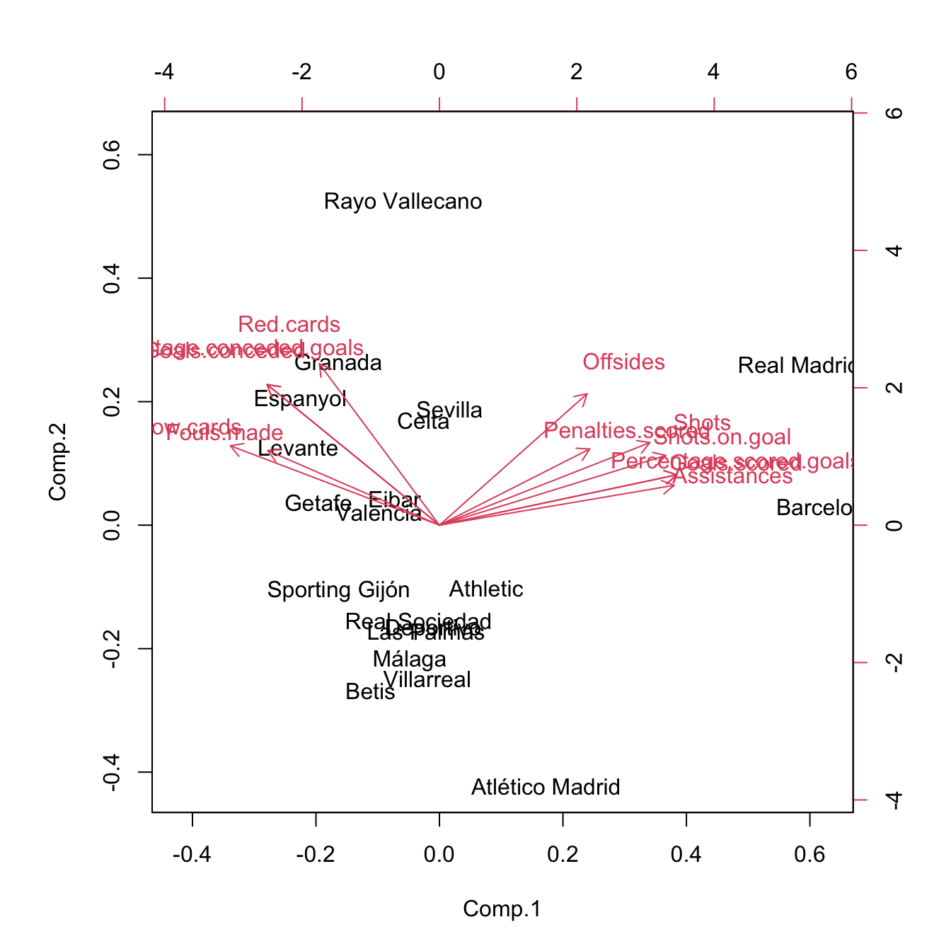

# PC1: attack performance of the team

# Create a new dataset with the response + principal components
laligaPCA <- data.frame("Points" = laliga$Points, pcaLaligaRed$scores)

# Regression on all the principal components
modPCA <- lm(Points ~ ., data = laligaPCA)
summary(modPCA) # Predictors clearly significative -- same R^2 as mod
## 
## Call:
## lm(formula = Points ~ ., data = laligaPCA)
## 
## Residuals:
##     Min      1Q  Median      3Q     Max 
## -5.2117 -1.4766  0.0544  1.9515  4.1422 
## 
## Coefficients:
##              Estimate Std. Error t value Pr(>|t|)    
## (Intercept)   52.4000     0.9557  54.831 1.76e-10 ***
## Comp.1         5.7690     0.3483  16.563 7.14e-07 ***
## Comp.2        -2.4376     0.6813  -3.578   0.0090 ** 
## Comp.3         3.4222     1.0443   3.277   0.0135 *  
## Comp.4        -3.6079     1.1141  -3.238   0.0143 *  
## Comp.5         1.9713     1.4535   1.356   0.2172    
## Comp.6         5.7067     1.7994   3.171   0.0157 *  
## Comp.7        -3.4169     2.8737  -1.189   0.2732    
## Comp.8         9.0212     3.6313   2.484   0.0419 *  
## Comp.9        -4.6455     6.5415  -0.710   0.5006    
## Comp.10      -10.2087     7.6299  -1.338   0.2227    
## Comp.11      222.0340   305.2920   0.727   0.4907    
## Comp.12     -954.7650   530.6164  -1.799   0.1150    
## ---
## Signif. codes:  0 '***' 0.001 '**' 0.01 '*' 0.05 '.' 0.1 ' ' 1
## 
## Residual standard error: 4.274 on 7 degrees of freedom
## Multiple R-squared:  0.9795, Adjusted R-squared:  0.9443 
## F-statistic: 27.83 on 12 and 7 DF,  p-value: 9.784e-05
car::vif(modPCA) # No problems at all
##  Comp.1  Comp.2  Comp.3  Comp.4  Comp.5  Comp.6  Comp.7  Comp.8  Comp.9 Comp.10 Comp.11 Comp.12 
##       1       1       1       1       1       1       1       1       1       1       1       1

# Using the first three components
modPCA3 <- lm(Points ~ Comp.1 + Comp.2 + Comp.3, data = laligaPCA)
summary(modPCA3)
## 
## Call:
## lm(formula = Points ~ Comp.1 + Comp.2 + Comp.3, data = laligaPCA)
## 
## Residuals:
##    Min     1Q Median     3Q    Max 
## -8.178 -4.541 -1.401  3.501 16.093 
## 
## Coefficients:
##             Estimate Std. Error t value Pr(>|t|)    
## (Intercept)  52.4000     1.5672  33.435 3.11e-16 ***
## Comp.1        5.7690     0.5712  10.100 2.39e-08 ***
## Comp.2       -2.4376     1.1173  -2.182   0.0444 *  
## Comp.3        3.4222     1.7126   1.998   0.0630 .  
## ---
## Signif. codes:  0 '***' 0.001 '**' 0.01 '*' 0.05 '.' 0.1 ' ' 1
## 
## Residual standard error: 7.009 on 16 degrees of freedom
## Multiple R-squared:  0.8738, Adjusted R-squared:  0.8501 
## F-statistic: 36.92 on 3 and 16 DF,  p-value: 2.027e-07

# Coefficients associated to each original predictor (gamma)
alpha <- modPCA3$coefficients
gamma <- pcaLaligaRed$loadings[, 1:3] %*% alpha[-1] # Slopes
gamma <- c(alpha[1] - pcaLaligaRed$center %*% gamma, gamma) # Intercept
names(gamma) <- c("Intercept", rownames(pcaLaligaRed$loadings))
gamma
##                 Intercept              Goals.scored            Goals.conceded   Percentage.scored.goals 
##               -44.2288551                 1.7305124                -3.4048178                 1.7416378 
## Percentage.conceded.goals                     Shots             Shots.on.goal          Penalties.scored 
##                -3.3944235                 0.2347716                 0.8782162                 2.6044699 
##               Assistances                Fouls.made              Yellow.cards                 Red.cards 
##                 1.4548813                -0.1171732                -1.7826488                -2.6423211 
##                  Offsides 
##                 1.3755697

# We can overpenalize to have a simpler model -- also one single
# principal component does quite well
modPCABIC <- MASS::stepAIC(modPCA, k = 2 * log(nrow(laliga)), trace = 0)
summary(modPCABIC)
## 
## Call:
## lm(formula = Points ~ Comp.1 + Comp.2 + Comp.3 + Comp.4 + Comp.6 + 
##     Comp.8, data = laligaPCA)
## 
## Residuals:
##     Min      1Q  Median      3Q     Max 
## -6.6972 -2.6418 -0.3265  2.3535  8.4944 
## 
## Coefficients:
##             Estimate Std. Error t value Pr(>|t|)    
## (Intercept)  52.4000     1.0706  48.946 3.95e-16 ***
## Comp.1        5.7690     0.3902  14.785 1.65e-09 ***
## Comp.2       -2.4376     0.7632  -3.194  0.00705 ** 
## Comp.3        3.4222     1.1699   2.925  0.01182 *  
## Comp.4       -3.6079     1.2481  -2.891  0.01263 *  
## Comp.6        5.7067     2.0158   2.831  0.01416 *  
## Comp.8        9.0212     4.0680   2.218  0.04502 *  
## ---
## Signif. codes:  0 '***' 0.001 '**' 0.01 '*' 0.05 '.' 0.1 ' ' 1
## 
## Residual standard error: 4.788 on 13 degrees of freedom
## Multiple R-squared:  0.9521, Adjusted R-squared:  0.9301 
## F-statistic: 43.11 on 6 and 13 DF,  p-value: 7.696e-08
# Note that the order of the principal components does not correspond
# exactly to its importance in the regression!

# To perform prediction we need to compute first the scores associated to the
# new values of the predictors, conveniently preprocessed
# Predictions for FCB and RMA (although they are part of the training sample)
newPredictors <- laligaRed[1:2, ]
newPredictors <- scale(newPredictors, center = pcaLaligaRed$center,
                       scale = pcaLaligaRed$scale) # Centered and scaled
newScores <- t(apply(newPredictors, 1,
                     function(x) t(pcaLaligaRed$loadings) %*% x))

# We need a data frame for prediction
newScores <- data.frame("Comp" = newScores)
predict(modPCABIC, newdata = newScores, interval = "prediction")
##                  fit      lwr      upr
## Barcelona   93.64950 80.35115 106.9478
## Real Madrid 90.05622 77.11876 102.9937

# Reality
laliga[1:2, 1]
## [1] 91 90

The second approach employs the function pls::pcr and is more direct, yet less connected with the techniques we have seen so far. It employs a model object that is different from the lm object and, as a consequence, functions like summary, BIC, MASS::stepAIC, or plot will not work properly. This implies that inference, model selection, and model diagnostics are not so straightforward. In exchange, pls::pcr allows for model fitting in an easier way and model selection through the use of cross-validation. In overall, this is a more pure predictive approach than predictive and explicative.

# Create a dataset without the problematic predictors and with the response
laligaRed2 <- subset(laliga, select = -c(Wins, Draws, Loses,
                                         Matches.without.conceding))

# Simple call to pcr
library(pls)
modPcr <- pcr(Points ~ ., data = laligaRed2, scale = TRUE)
# Notice we do not need to create a data.frame with PCA, it is automatically
# done within pcr. We also have flexibility to remove predictors from the PCA
# scale = TRUE means that the predictors are scaled internally before computing
# PCA

# The summary of the model is different
summary(modPcr)
## Data:    X dimension: 20 12 
##  Y dimension: 20 1
## Fit method: svdpc
## Number of components considered: 12
## TRAINING: % variance explained
##         1 comps  2 comps  3 comps  4 comps  5 comps  6 comps  7 comps  8 comps  9 comps  10 comps  11 comps  12 comps
## X         62.73    79.13    86.11    92.24    95.84    98.19    99.11    99.69    99.87    100.00       100    100.00
## Points    80.47    84.23    87.38    90.45    90.99    93.94    94.36    96.17    96.32     96.84        97     97.95
# First row: percentage of variance explained of the predictors
# Second row: percentage of variance explained of Y (the R^2)
# Note that we have the same R^2 for 3 and 12 components as in the previous
# approach

# Slots of information in the model -- most of them as 3-dim arrays with the
# third dimension indexing the number of components considered
names(modPcr)
##  [1] "coefficients"  "scores"        "loadings"      "Yloadings"     "projection"    "Xmeans"        "Ymeans"       
##  [8] "fitted.values" "residuals"     "Xvar"          "Xtotvar"       "fit.time"      "ncomp"         "method"       
## [15] "center"        "scale"         "call"          "terms"         "model"

# The coefficients of the original predictors (gammas), not of the components!
modPcr$coefficients[, , 12]
##              Goals.scored            Goals.conceded   Percentage.scored.goals Percentage.conceded.goals 
##             -602.85050765             -383.07010184              600.61255371              374.38729000 
##                     Shots             Shots.on.goal          Penalties.scored               Assistances 
##               -8.27239221                0.88174787               -2.14313238               24.42240486 
##                Fouls.made              Yellow.cards                 Red.cards                  Offsides 
##               -2.96044265                5.51983512                1.20945331               -0.07231723
# pcr() computes up to ncomp (in this case, 12) linear models, each one
# considering one extra principal component. $coefficients returns in a
# 3-dim array the coefficients of all the linear models

# Prediction is simpler and can be done for different number of components
predict(modPcr, newdata = laligaRed2[1:2, ], ncomp = 12)
## , , 12 comps
## 
##               Points
## Barcelona   92.01244
## Real Madrid 91.38026

# Selecting the number of components to retain. All the components up to ncomp
# are selected, no further flexibility is possible
modPcr2 <- pcr(Points ~ ., data = laligaRed2, scale = TRUE, ncomp = 3)
summary(modPcr2)
## Data:    X dimension: 20 12 
##  Y dimension: 20 1
## Fit method: svdpc
## Number of components considered: 3
## TRAINING: % variance explained
##         1 comps  2 comps  3 comps
## X         62.73    79.13    86.11
## Points    80.47    84.23    87.38

# Selecting the number of components to retain by Leave-One-Out
# cross-validation
modPcrCV1 <- pcr(Points ~ ., data = laligaRed2, scale = TRUE,
                 validation = "LOO")
summary(modPcrCV1)
## Data:    X dimension: 20 12 
##  Y dimension: 20 1
## Fit method: svdpc
## Number of components considered: 12
## 
## VALIDATION: RMSEP
## Cross-validated using 20 leave-one-out segments.
##        (Intercept)  1 comps  2 comps  3 comps  4 comps  5 comps  6 comps  7 comps  8 comps  9 comps  10 comps  11 comps
## CV           18.57    8.505    8.390    8.588    7.571    7.688    6.743     7.09    6.224    6.603     7.547     8.375
## adjCV        18.57    8.476    8.356    8.525    7.513    7.663    6.655     7.03    6.152    6.531     7.430     8.236
##        12 comps
## CV        7.905
## adjCV     7.760
## 
## TRAINING: % variance explained
##         1 comps  2 comps  3 comps  4 comps  5 comps  6 comps  7 comps  8 comps  9 comps  10 comps  11 comps  12 comps
## X         62.73    79.13    86.11    92.24    95.84    98.19    99.11    99.69    99.87    100.00       100    100.00
## Points    80.47    84.23    87.38    90.45    90.99    93.94    94.36    96.17    96.32     96.84        97     97.95

# View cross-validation Mean Squared Error in Prediction
validationplot(modPcrCV1, val.type = "MSEP") # l = 8 gives the minimum CV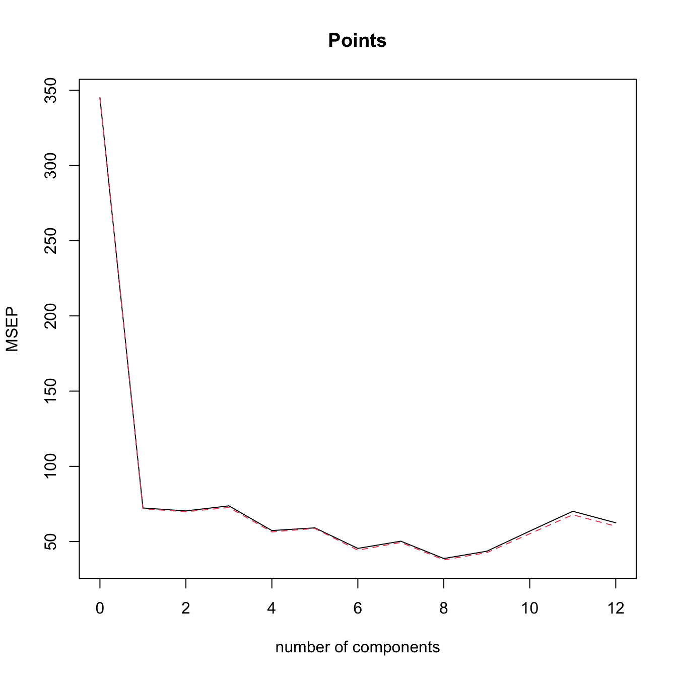

# The black is the CV loss, the dashed red line is the adjCV loss, a bias
# corrected version of the MSEP (not described in the notes)

# Selecting the number of components to retain by 10-fold Cross-Validation
# (k = 10 is the default, this can be changed with the argument segments)
modPcrCV10 <- pcr(Points ~ ., data = laligaRed2, scale = TRUE,
                  validation = "CV")
summary(modPcrCV10)
## Data:    X dimension: 20 12 
##  Y dimension: 20 1
## Fit method: svdpc
## Number of components considered: 12
## 
## VALIDATION: RMSEP
## Cross-validated using 10 random segments.
##        (Intercept)  1 comps  2 comps  3 comps  4 comps  5 comps  6 comps  7 comps  8 comps  9 comps  10 comps  11 comps
## CV           18.57    8.520    8.392    8.911    7.187    7.124    6.045    6.340    5.728    6.073     7.676     9.300
## adjCV        18.57    8.464    8.331    8.768    7.092    7.043    5.904    6.252    5.608    5.953     7.423     8.968
##        12 comps
## CV        9.151
## adjCV     8.782
## 
## TRAINING: % variance explained
##         1 comps  2 comps  3 comps  4 comps  5 comps  6 comps  7 comps  8 comps  9 comps  10 comps  11 comps  12 comps
## X         62.73    79.13    86.11    92.24    95.84    98.19    99.11    99.69    99.87    100.00       100    100.00
## Points    80.47    84.23    87.38    90.45    90.99    93.94    94.36    96.17    96.32     96.84        97     97.95
validationplot(modPcrCV10, val.type = "MSEP") # l = 8 gives the minimum CV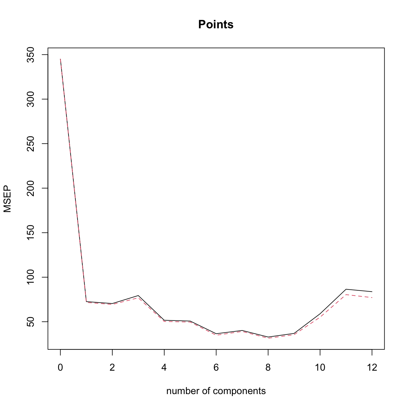

pcr() does an internal scaling of the predictors by their quasi-standard deviations. This means that each variable is divided by \(\frac{1}{\sqrt{n-1}},\) when in princomp a scaling of \(\frac{1}{\sqrt{n}}\) is applied (the standard deviations are employed). This results in a minor discrepancy in the scores object of both methods that is easily patchable. The scores of princomp() are the ones of pcr() multiplied by \(\sqrt{\frac{n}{n-1}}.\) This problem is inherited to the coefficients, which assume scores divided by \(\frac{1}{\sqrt{n-1}}.\) Therefore, the \(\hat{\boldsymbol{\gamma}}\) coefficients described in (3.16) are obtained by dividing the coefficients of pcr() by \(\sqrt{\frac{n}{n-1}}.\)

The next chunk of code illustrates the previous warning.

# Equality of loadings from princomp() and pcr()
max(abs(abs(pcaLaligaRed$loadings[, 1:3]) - abs(modPcr$loadings[, 1:3])))
## [1] 2.664535e-15

# Equality of scores from princomp() and pcr() (with the same standardization)
max(abs(abs(pcaLaligaRed$scores[, 1:3]) -
          abs(modPcr$scores[, 1:3] * sqrt(n / (n - 1)))))
## [1] 9.298118e-15

# Equality of the gamma coefficients obtained previously for 3 PCA
# (with the same standardization)
modPcr$coefficients[, , 3] / sqrt(n / (n - 1))
##              Goals.scored            Goals.conceded   Percentage.scored.goals Percentage.conceded.goals 
##                 1.7305124                -3.4048178                 1.7416378                -3.3944235 
##                     Shots             Shots.on.goal          Penalties.scored               Assistances 
##                 0.2347716                 0.8782162                 2.6044699                 1.4548813 
##                Fouls.made              Yellow.cards                 Red.cards                  Offsides 
##                -0.1171732                -1.7826488                -2.6423211                 1.3755697
gamma[-1]
##              Goals.scored            Goals.conceded   Percentage.scored.goals Percentage.conceded.goals 
##                 1.7305124                -3.4048178                 1.7416378                -3.3944235 
##                     Shots             Shots.on.goal          Penalties.scored               Assistances 
##                 0.2347716                 0.8782162                 2.6044699                 1.4548813 
##                Fouls.made              Yellow.cards                 Red.cards                  Offsides 
##                -0.1171732                -1.7826488                -2.6423211                 1.3755697

# Coefficients associated to the principal components -- same as in modPCA3
lm(Points ~ ., data = data.frame("Points" = laliga$Points,
                                 modPcr$scores[, 1:3] * sqrt(n / (n - 1))))
## 
## Call:
## lm(formula = Points ~ ., data = data.frame(Points = laliga$Points, 
##     modPcr$scores[, 1:3] * sqrt(n/(n - 1))))
## 
## Coefficients:
## (Intercept)       Comp.1       Comp.2       Comp.3  
##      52.400       -5.769        2.438       -3.422
modPCA3
## 
## Call:
## lm(formula = Points ~ Comp.1 + Comp.2 + Comp.3, data = laligaPCA)
## 
## Coefficients:
## (Intercept)       Comp.1       Comp.2       Comp.3  
##      52.400        5.769       -2.438        3.422
# Of course, flipping of signs is always possible with PCA

The selection of \(\ell\) by cross-validation attempts to minimize the Mean Squared Error in Prediction (MSEP) or, equivalently, the Root MSEP (RMSEP) of the model⁹⁶. This is a Swiss army knife method valid for the selection of any tuning parameter \(\lambda\) that affects the form of the estimate \(\hat{m}_\lambda\) of the regression function \(m\) (remember (1.1)). Given the sample \(\{(\mathbf{X}_i,Y_i)\}_{i=1}^n,\) leave-one-out cross-validation considers the tuning parameter

\[\begin{align} \hat{\lambda}_\text{CV}:=\arg\min_{\lambda\geq0} \sum_{i=1}^n (Y_i-\hat{m}_{\lambda,-i}(\mathbf{X}_i))^2,\tag{3.17} \end{align}\]

where \(\hat{m}_{\lambda,-i}\) represents the fit of the model \(\hat{m}_\lambda\) without the \(i\)-th observation \((\mathbf{X}_i,Y_i).\)

A less computationally expensive variation on leave-one-out cross-validation is \(k\)-fold cross-validation, which partitions the data into \(k\) folds \(F_1,\ldots, F_k\) of approximately equal size, trains the model \(\hat{m}_\lambda\) in the aggregation of \(k-1\) folds, and evaluates its MSEP in the remaining fold:

\[\begin{align} \hat{\lambda}_{k\text{-CV}}:=\arg\min_{\lambda\geq0} \sum_{j=1}^k \sum_{i\in F_j} (Y_i-\hat{m}_{\lambda,-F_{j}}(\mathbf{X}_i))^2,\tag{3.18} \end{align}\]

where \(\hat{m}_{\lambda,-F_{j}}\) represents the fit of the model \(\hat{m}_\lambda\) excluding the data from the \(j\)-th fold \(F_{j}.\) Recall that \(k\)-fold cross-validation is more general than leave-one-out cross-validation, since the latter is a particular case of the former with \(k=n.\)

\(k\)-fold cross validation with \(k<n\) depends on the choice of the folds for splitting the data (i.e., how each datum is assigned to each of the \(k\) folds). Some statistical softwares do this assignment randomly, which means that the selection of \(\hat{\lambda}_{k\text{-CV}}\) may vary from one run to another. Thus, fixing the seed prior to the parameter selection is important to ensure reproducibility. Another alternative is to aggregate, in a convenient way, the results of several \(k\)-fold cross-validations done in different random random partitions. This problem is not present in leave-one-out cross-validation (where \(k=n\)).

Inference in PCR can be carried out as in the standard linear model. The key point is to realize that it is about the coefficients \(\boldsymbol{\alpha}_{0:\ell}\) associated to the \(\ell\) principal components, and that it can be carried out by the summary() function on the output of lm(). The coefficients \(\boldsymbol{\alpha}_{0:\ell}\) are the ones estimated by least squares when considering the scores of the \(\ell\) principal components as the predictors. This transformation of the predictors does not affect the validity of the inferential results of Section 2.4 (derived conditionally on the predictors). But recall that this inference is not about \(\boldsymbol{\gamma}.\)

Inference in PCR is based on the assumptions of the linear model being satisfied for the considered conprincipal components. The evaluation of the assumptions can be done using the exact same tools described in Section 3.5. However, keep in mind that PCA is a linear transformation of the data. Therefore:

• If the linearity assumption fails for the predictors \(X_1,\ldots,X_p,\) then it will also likely fail for \(\Gamma_1,\ldots,\Gamma_\ell,\) since the transformation will not introduce nonlinearities able to capture the nonlinear effects.
• Similarly, if the homoscedasticity, normality, or independence assumptions fail for \(X_1,\ldots,X_p,\) then they will also likely fail for \(\Gamma_1,\ldots,\Gamma_\ell.\)

Exceptions to the previous common implications are possible, and may involve the association of one or several problematic predictors (e.g., have nonlinear effects on the response) to the principal components that are excluded from the model. Up to which extent the failure of the assumptions in the original predictors can be mitigated by PCR depends on each application.

3.6.3 Partial least squares regression

PCR works by replacing the predictors \(X_1,\ldots,X_p\) by a set of principal components \(\Gamma_1,\ldots,\Gamma_\ell,\) under the hope that these directions, that explain most of the variability of the predictors, are also the best directions for predicting the response \(Y.\) While this is a reasonable belief, it is not a guaranteed fact. Partial Least Squares Regression (PLSR) precisely tackles this point with the idea of regressing the response \(Y\) on a set of new variables \(P_1,\ldots,P_\ell\) that are constructed with the objective of predicting \(Y\) from \(X_1,\ldots,X_p\) in the best linear way.

As with PCA, the idea is to find linear combinations of the predictors \(X_1,\ldots,X_p,\) that is, to have:

\[\begin{align} P_1:=\sum_{j=1}^pa_{1j}X_j,\,\ldots,\,P_p:=\sum_{j=1}^pa_{pj}X_j.\tag{3.19} \end{align}\]

These new predictors are called PLS components⁹⁷.

The question is how to choose the coefficients \(a_{kj},\) \(j,k=1,\ldots,p.\) PLSR does it by placing the most weight in the predictors that are most strongly correlated with \(Y\) and in such a way that the resulting \(P_1,\ldots,P_p\) are uncorrelated between them. After standardizing the variables, for \(P_1\) this is achieved by setting \(a_{1j}\) equal to the theoretical slope coefficient of regressing \(Y\) into \(X_j,\) that is⁹⁸:

\[\begin{align*} a_{1j}:=\frac{\mathrm{Cov}[X_j,Y]}{\mathbb{V}\mathrm{ar}[X_j]}, \end{align*}\]

where \(a_{1j}\) stems from \(Y=a_{0}+a_{1j}X_j+\varepsilon.\)

The second partial least squares direction, \(P_2,\) is computed in a similar way, but once the linear effects of \(P_1\) on \(X_1,\ldots,X_p\) are removed. This is achieved by:

1. Regressing each of \(X_1,\ldots,X_p\) on \(P_1.\) That is, fit the \(p\) simple linear models

\[\begin{align*} X_j=\alpha_0+\alpha_{1j}P_1+\varepsilon_j,\quad j=1,\ldots,p. \end{align*}\]

2. Regress \(Y\) on each of the \(p\) random errors \(\varepsilon_{1},\ldots,\varepsilon_{p}\;\)⁹⁹ from the above regressions, yielding

   \[\begin{align*} a_{2j}:=\frac{\mathrm{Cov}[\varepsilon_j,Y]}{\mathbb{V}\mathrm{ar}[\varepsilon_j]}, \end{align*}\]

   where \(a_{2j}\) stems from \(Y=a_{0}+a_{2j}\varepsilon_j+\varepsilon.\)

The coefficients for \(P_j,\) \(j>2,\) are computed¹⁰⁰ by iterating the former process. Once \(P_1,\ldots,P_\ell\) are obtained, then PLSR proceeds as PCR and fits the model

\[\begin{align*} Y=\beta_0+\beta_1P_1+\cdots+\beta_\ell P_\ell+\varepsilon. \end{align*}\]

The implementation of PLSR can be done by the function pls::plsr, which has an analogous syntax to pls::pcr.

# Simple call to plsr -- very similar to pcr
modPlsr <- plsr(Points ~ ., data = laligaRed2, scale = TRUE)

# The summary of the model
summary(modPlsr)
## Data:    X dimension: 20 12 
##  Y dimension: 20 1
## Fit method: kernelpls
## Number of components considered: 12
## TRAINING: % variance explained
##         1 comps  2 comps  3 comps  4 comps  5 comps  6 comps  7 comps  8 comps  9 comps  10 comps  11 comps  12 comps
## X         62.53    76.07    84.94    88.29    92.72    95.61    98.72    99.41    99.83    100.00    100.00    100.00
## Points    83.76    91.06    93.93    95.43    95.94    96.44    96.55    96.73    96.84     96.84     97.69     97.95
# First row: percentage of variance explained of the predictors
# Second row: percentage of variance explained of Y (the R^2)
# Note we have the same R^2 for 12 components as in the linear model

# Slots of information in the model
names(modPlsr)
##  [1] "coefficients"    "scores"          "loadings"        "loading.weights" "Yscores"         "Yloadings"      
##  [7] "projection"      "Xmeans"          "Ymeans"          "fitted.values"   "residuals"       "Xvar"           
## [13] "Xtotvar"         "fit.time"        "ncomp"           "method"          "center"          "scale"          
## [19] "call"            "terms"           "model"

# PLS scores
head(modPlsr$scores)
##                      Comp 1     Comp 2     Comp 3     Comp 4     Comp 5      Comp 6     Comp 7     Comp 8      Comp 9
## Barcelona        7.36407868 -0.6592285 -0.4262822 -0.1357589  0.8668796 -0.52701770 -0.1547704 -0.3104798 -0.15841110
## Real Madrid      6.70659816 -1.2848902  0.7191143  0.5679398 -0.5998745  0.30663290  0.5382173  0.2110337  0.15242836
## Atlético Madrid  2.45577740  2.6469837  0.4573647  0.6179274 -0.4307465  0.13368949  0.2951566 -0.1597672 -0.15232469
## Villarreal       0.06913485  2.0275895  0.6548014 -0.2358589  0.8350426  0.61305618 -0.6684330  0.0556628  0.07919102
## Athletic         0.96513341  0.3860060 -0.2718465 -0.1580349 -0.2649106  0.01822319 -0.1899969  0.3846156 -0.28926416
## Celta           -0.39588401 -0.5296417  0.6148093  0.1494496  0.5817902  0.69106828  0.1586472  0.2396975  0.41575546
##                     Comp 10       Comp 11       Comp 12
## Barcelona       -0.18952142 -0.0001005279  0.0011993985
## Real Madrid      0.15826286 -0.0011752690 -0.0030013550
## Atlético Madrid  0.05857664  0.0028149603  0.0012838990
## Villarreal      -0.05343433  0.0012705829 -0.0001652195
## Athletic         0.03702926 -0.0008077855  0.0052995290
## Celta           -0.03488514  0.0003208900  0.0022585552

# Also uncorrelated
head(cov(modPlsr$scores))
##               Comp 1        Comp 2        Comp 3        Comp 4        Comp 5        Comp 6        Comp 7        Comp 8
## Comp 1  7.393810e+00  3.973430e-16 -2.337312e-16 -7.304099e-18  9.115515e-16  1.149665e-15  3.272236e-16  7.011935e-17
## Comp 2  3.973430e-16  1.267859e+00 -2.980072e-16 -1.840633e-16 -2.103580e-16 -1.920978e-16 -2.337312e-17 -9.495329e-17
## Comp 3 -2.337312e-16 -2.980072e-16  9.021126e-01 -8.399714e-18  1.256305e-16  1.003401e-16 -2.921640e-18  5.843279e-18
## Comp 4 -7.304099e-18 -1.840633e-16 -8.399714e-18  3.130984e-01 -5.660677e-17 -4.660928e-17 -3.652049e-19  2.282531e-17
## Comp 5  9.115515e-16 -2.103580e-16  1.256305e-16 -5.660677e-17  2.586132e-01  9.897054e-17  8.180591e-17  3.432926e-17
## Comp 6  1.149665e-15 -1.920978e-16  1.003401e-16 -4.660928e-17  9.897054e-17  2.792408e-01  1.132135e-17  1.314738e-17
##               Comp 9       Comp 10       Comp 11       Comp 12
## Comp 1 -4.090295e-17 -2.571043e-16 -1.349090e-16 -3.928806e-16
## Comp 2 -1.358562e-16 -3.652049e-17 -1.000234e-16  2.990686e-17
## Comp 3 -1.168656e-17 -2.848599e-17  8.478176e-18 -9.205732e-18
## Comp 4  2.246010e-17  2.757297e-17 -2.658007e-17 -7.249889e-18
## Comp 5  4.382459e-18  1.679943e-17 -5.937433e-18  7.983152e-18
## Comp 6  1.150396e-17  2.191230e-18 -2.137412e-17 -5.567770e-18

# The coefficients of the original predictors, not of the components!
modPlsr$coefficients[, , 2]
##              Goals.scored            Goals.conceded   Percentage.scored.goals Percentage.conceded.goals 
##                 1.8192870                -4.4038213                 1.8314760                -4.4045722 
##                     Shots             Shots.on.goal          Penalties.scored               Assistances 
##                 0.4010902                 0.9369002                -0.2006251                 2.3688050 
##                Fouls.made              Yellow.cards                 Red.cards                  Offsides 
##                 0.2807601                -1.6677725                -2.4952503                 1.2187529

# Obtaining the coefficients of the PLS components
lm(formula = Points ~., data = data.frame("Points" = laliga$Points,
                                          modPlsr$scores[, 1:3]))
## 
## Call:
## lm(formula = Points ~ ., data = data.frame(Points = laliga$Points, 
##     modPlsr$scores[, 1:3]))
## 
## Coefficients:
## (Intercept)       Comp.1       Comp.2       Comp.3  
##      52.400        6.093        4.341        3.232

# Prediction
predict(modPlsr, newdata = laligaRed2[1:2, ], ncomp = 12)
## , , 12 comps
## 
##               Points
## Barcelona   92.01244
## Real Madrid 91.38026

# Selecting the number of components to retain
modPlsr2 <- plsr(Points ~ ., data = laligaRed2, scale = TRUE, ncomp = 2)
summary(modPlsr2)
## Data:    X dimension: 20 12 
##  Y dimension: 20 1
## Fit method: kernelpls
## Number of components considered: 2
## TRAINING: % variance explained
##         1 comps  2 comps
## X         62.53    76.07
## Points    83.76    91.06

# Selecting the number of components to retain by Leave-One-Out cross-validation
modPlsrCV1 <- plsr(Points ~ ., data = laligaRed2, scale = TRUE,
                   validation = "LOO")
summary(modPlsrCV1)
## Data:    X dimension: 20 12 
##  Y dimension: 20 1
## Fit method: kernelpls
## Number of components considered: 12
## 
## VALIDATION: RMSEP
## Cross-validated using 20 leave-one-out segments.
##        (Intercept)  1 comps  2 comps  3 comps  4 comps  5 comps  6 comps  7 comps  8 comps  9 comps  10 comps  11 comps
## CV           18.57    8.307    7.221    6.807    6.254    6.604    6.572    6.854    7.348    7.548     7.532     7.854
## adjCV        18.57    8.282    7.179    6.742    6.193    6.541    6.490    6.764    7.244    7.430     7.416     7.717
##        12 comps
## CV        7.905
## adjCV     7.760
## 
## TRAINING: % variance explained
##         1 comps  2 comps  3 comps  4 comps  5 comps  6 comps  7 comps  8 comps  9 comps  10 comps  11 comps  12 comps
## X         62.53    76.07    84.94    88.29    92.72    95.61    98.72    99.41    99.83    100.00    100.00    100.00
## Points    83.76    91.06    93.93    95.43    95.94    96.44    96.55    96.73    96.84     96.84     97.69     97.95

# View cross-validation Mean Squared Error Prediction
validationplot(modPlsrCV1, val.type = "MSEP") # l = 4 gives the minimum CV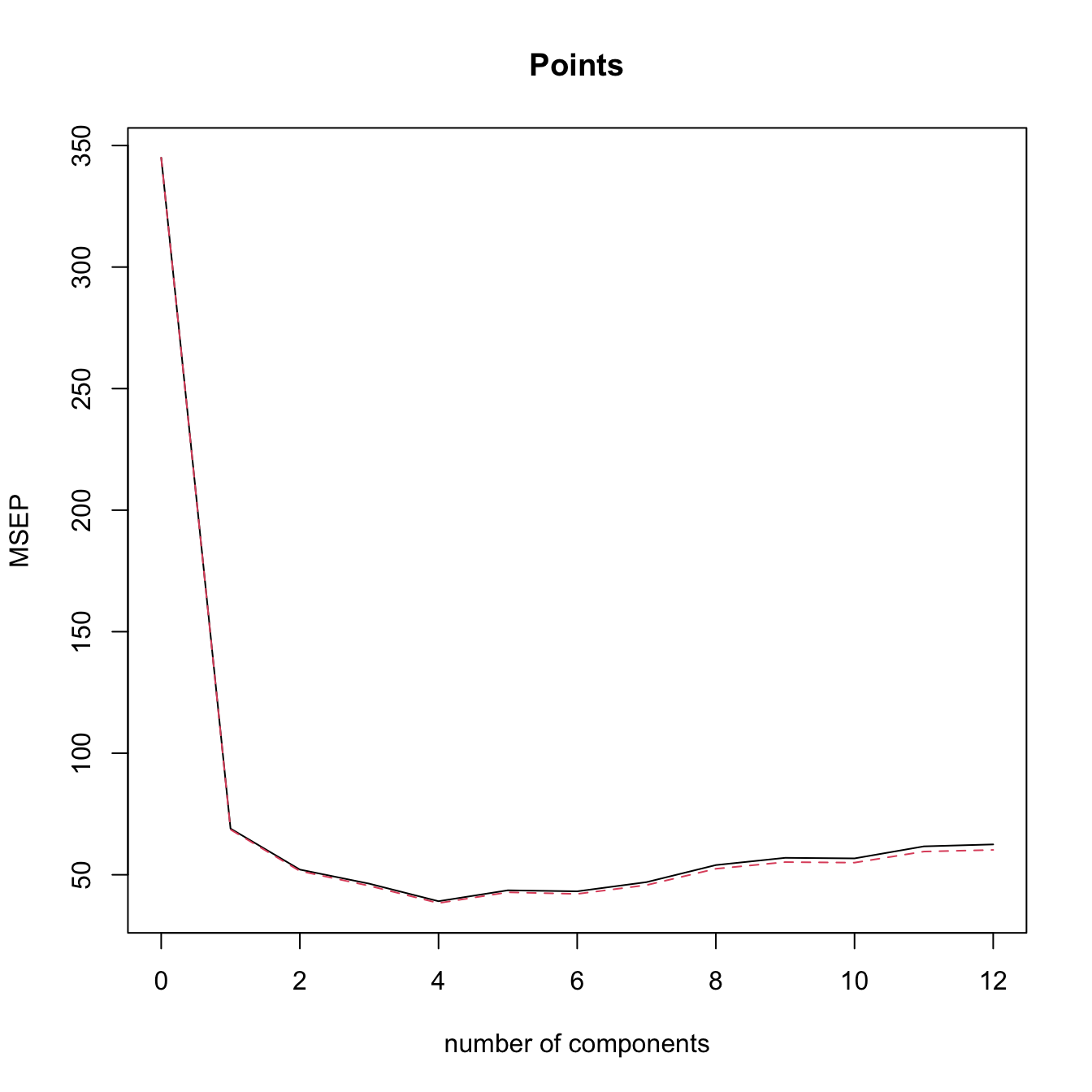

# Selecting the number of components to retain by 10-fold Cross-Validation
# (k = 10 is the default)
modPlsrCV10 <- plsr(Points ~ ., data = laligaRed2, scale = TRUE,
                    validation = "CV")
summary(modPlsrCV10)
## Data:    X dimension: 20 12 
##  Y dimension: 20 1
## Fit method: kernelpls
## Number of components considered: 12
## 
## VALIDATION: RMSEP
## Cross-validated using 10 random segments.
##        (Intercept)  1 comps  2 comps  3 comps  4 comps  5 comps  6 comps  7 comps  8 comps  9 comps  10 comps  11 comps
## CV           18.57    7.895    6.944    6.571    6.330    6.396    6.607    7.018    7.487    7.612     7.607     8.520
## adjCV        18.57    7.852    6.868    6.452    6.201    6.285    6.444    6.830    7.270    7.372     7.368     8.212
##        12 comps
## CV        8.014
## adjCV     7.714
## 
## TRAINING: % variance explained
##         1 comps  2 comps  3 comps  4 comps  5 comps  6 comps  7 comps  8 comps  9 comps  10 comps  11 comps  12 comps
## X         62.53    76.07    84.94    88.29    92.72    95.61    98.72    99.41    99.83    100.00    100.00    100.00
## Points    83.76    91.06    93.93    95.43    95.94    96.44    96.55    96.73    96.84     96.84     97.69     97.95
validationplot(modPlsrCV10, val.type = "MSEP")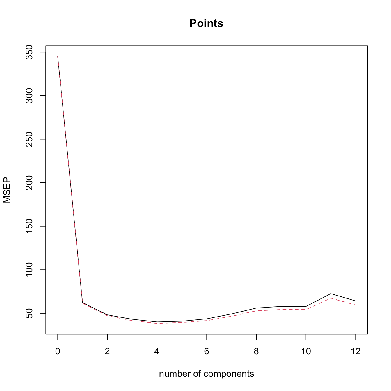

# l = 4 is close to the minimum CV

# Regress manually Points in the scores, in order to have an lm object
# Create a new dataset with the response + PLS components
laligaPLS <- data.frame("Points" = laliga$Points, cbind(modPlsr$scores))

# Regression on the first two PLS
modPlsr <- lm(Points ~ Comp.1 + Comp.2, data = laligaPLS)
summary(modPlsr) # Predictors clearly significative -- same R^2 as in modPlsr2
## 
## Call:
## lm(formula = Points ~ Comp.1 + Comp.2, data = laligaPLS)
## 
## Residuals:
##     Min      1Q  Median      3Q     Max 
## -9.3565 -3.6157  0.4508  2.3288 12.3116 
## 
## Coefficients:
##             Estimate Std. Error t value Pr(>|t|)    
## (Intercept)  52.4000     1.2799  40.941  < 2e-16 ***
## Comp.1        6.0933     0.4829  12.618 4.65e-10 ***
## Comp.2        4.3413     1.1662   3.723  0.00169 ** 
## ---
## Signif. codes:  0 '***' 0.001 '**' 0.01 '*' 0.05 '.' 0.1 ' ' 1
## 
## Residual standard error: 5.724 on 17 degrees of freedom
## Multiple R-squared:  0.9106, Adjusted R-squared:    0.9 
## F-statistic: 86.53 on 2 and 17 DF,  p-value: 1.225e-09
car::vif(modPlsr) # No problems at all
## Comp.1 Comp.2 
##      1      1

Let’s perform PCR and PLSR in the iris dataset. Recall that this dataset contains a factor variable, which can not be treated directly by princomp but can be used in PCR/PLSR (it is transformed internally to two dummy variables). Do the following:

1. Compute the PCA of iris, excluding Species. What is the percentage of variability explained with two components?
2. Draw the biplot and look for interpretations of the principal components.
3. Plot the PCA scores in a car::scatterplotMatrix plot such that the scores are colored by the levels in Species (you can use the groups argument).
4. Compute the PCR of Petal.Width with \(\ell=2\) (exclude Species). Inspect by leave-one-out cross-validation the best selection of \(\ell.\)
5. Repeat the previous point with PLSR.
6. Plot the PLS scores of the data in a car::scatterplotMatrix plot such that the scores are colored by the levels in Species. Compare with the PCA scores. Is there any interesting interpretation? (A quick way of converting the scores to a matrix is with rbind.)

In theory, the dimensionality reduction of PLSR is more adequate for linear regression than that of PCR. However, in many practical situations PLSR and PCR tend to perform similarly, since the variance of the PLSR predictors \(P_1,\ldots,P_\ell\) is larger (due to the iterative linear-filtering procedure on which they are constructed) than the variance of the PCR predictors \(\Gamma_1,\ldots,\Gamma_\ell.\)

Inference for PLSR is more involved since, differently to what happens in PCR, the PLS directions are dependent on the response \(Y\). This directly breaks a core assumption made in Section 2.4: that the randomness of the regression model came only from the error terms and not from the predictors.

We conclude by illustrating the differences between PLSR and PCR with a small numerical example. For that, we consider two correlated predictors \[\begin{align} \begin{pmatrix}X_1\\X_2\end{pmatrix}\sim \mathcal{N}_2\left(\begin{pmatrix}0\\0\end{pmatrix},\begin{pmatrix}1&\rho\\\rho&1\end{pmatrix}\right), \quad -1\leq\rho\leq1,\tag{3.20} \end{align}\] and the linear model \[\begin{align} Y=\beta_1X_1+\beta_2X_2+\varepsilon,\quad \boldsymbol{\beta}=\begin{pmatrix}\cos(\theta)\\\sin(\theta)\end{pmatrix},\tag{3.21} \end{align}\] where \(\theta\in[0,2\pi)\) and \(\varepsilon\sim\mathcal{N}(0,1).\) Therefore:

• The correlation \(\rho\) controls the linear dependence between \(X_1\) and \(X_2\). This parameter is the only one that affects the two principal components \(\Gamma_1=a_{11}X_1+a_{21}X_2\) and \(\Gamma_2=a_{12}X_1+a_{22}X_2\) (recall (3.9)). The loadings \((\hat{a}_{11},\hat{a}_{21})'\) and \((\hat{a}_{12},\hat{a}_{22})'\) are the (sample) PC1 and PC2 directions.
• The angle \(\theta\) controls the direction of \(\boldsymbol{\beta},\) that is, the linear relation between \(Y\) and \((X_1,X_2)\). Consequently, \(\theta\) affects the PLS components \(P_1=b_{11}X_1+b_{21}X_2\) and \(P_2=b_{12}X_1+b_{22}X_2\) (recall (3.19), with adapted notation). The loadings \((\hat{b}_{11},\hat{b}_{21})'\) and \((\hat{b}_{12},\hat{b}_{22})'\) are the (sample) PLS1 and PLS2 directions.

The animation in Figure 3.35 contains samples from (3.20) colored according to their expected value under (3.21). It illustrates the following insights:

• PC directions are unaware of \(\boldsymbol{\beta};\) PLS directions are affected by \(\boldsymbol{\beta}.\)
• PC directions are always orthogonal; PLS directions are not.
• PLS1 aligns¹⁰¹ with \(\boldsymbol{\beta}\) when \(\rho = 0.\) This does not happen when \(\rho \neq 0\) (remember Figure 2.7).
• Under high correlation, the PLS and PC directions are very similar.
• Under low-moderate correlation, PLS1 better explains¹⁰² \(\boldsymbol{\beta}\) than PC1.

Figure 3.35: Illustration of the differences and similarities between PCR and PLSR. The points are sampled from (3.20) and colored according to their expected value under (3.21): yellow for larger values; dark violet for smaller. The color gradient is thus controlled by the direction of \(\boldsymbol{\beta}\) (black arrow) and informs on the position of the plane \(y=\beta_1x_1+\beta_2x_2.\) The PC/PLS directions are described in the text. Application available here.

---

80. That is, \(\mathbb{E}[X_j]=0,\) \(j=1,\ldots,p.\) This is important since PCA is sensitive to the centering of the data.↩︎

81. Recall that the covariance matrix is a real, symmetric, semi-positive definite matrix.↩︎

82. Therefore, \(\mathbf{A}^{-1}=\mathbf{A}'.\)↩︎

83. Since the variance-covariance matrix \(\mathbb{V}\mathrm{ar}[\boldsymbol{\Gamma}]\) is diagonal.↩︎

84. Up to now, the exposition has been focused exclusively on the population case.↩︎

85. Some care is needed here. The matrix \(\mathbf{S}\) is obtained from linear combinations of the \(n\) vectors \(\mathbf{X}_1-\bar{\mathbf{X}},\ldots,\mathbf{X}_n-\bar{\mathbf{X}}.\) Recall that these \(n\) vectors are not linearly independent, as they are guaranteed to add \(\mathbf{0},\) \(\sum_{i=1}^n[\mathbf{X}_i-\bar{\mathbf{X}}]=\mathbf{0},\) so it is possible to express one perfectly on the rest. That implies that the \(p\times p\) matrix \(\mathbf{S}\) has rank smaller or equal to \(n-1.\) If \(p\leq n-1,\) then the matrix has full rank \(p\) and it is invertible (excluding degenerate cases in which the \(p\) variables are collinear). But if \(p\geq n,\) then \(\mathbf{S}\) is singular and, as a consequence, \(\lambda_j=0\) for \(j\geq n.\) This implies that the principal components for those eigenvalues cannot be determined univocally.↩︎

86. Therefore, a sample of lengths measured in centimeters will have a variance \(10^4\) times larger than the same sample measured in meters – yet it is the same information!↩︎

87. The biplot is implemented in R by biplot.princomp (or by biplot applied to a princomp object). This function applies an internal scaling of the scores and variables to improve the visualization (see ?biplot.princomp), which can be disabled with the argument scale = 0.↩︎

88. For the sample version, replace the variable \(X_j\) by its sample \(X_{1j},\ldots,X_{nj},\) the loadings \(a_{ji}\) by their estimates \(\hat a_{ji},\) and the principal component \(\Gamma_j\) by the scores \(\{\hat{\Gamma}_{ij}\}_{i=1}^n.\)↩︎

89. Observe that both \(X_j=a_{j1}\Gamma_{1} + a_{j2}\Gamma_{2} + \cdots + a_{jp}\Gamma_{p}\) and \(\Gamma_j=a_{1j}X_{1} + a_{2j}X_{2} + \cdots + a_{pj}X_{p},\) \(j=1,\ldots,p,\) hold simultaneously due to the orthogonality of \(\mathbf{A}.\)↩︎

90. The first two principal components of the dataset explain the \(78\%\) of the variability of the data. Hence, the insights obtained from the biplot should be regarded as “\(78\%\)-accurate”.↩︎

91. This is certainly not always true, but it is often the case. See Figure 3.35.↩︎

92. For the sake of simplicity, we considering the exposition the first \(\ell\) principal components, but obviously other combinations of \(\ell\) principal components are possible.↩︎

93. Since we know by (3.11) that \(\boldsymbol{\Gamma}=\mathbf{A}'(\mathbf{X}-\boldsymbol{\mu}),\) where \(\mathbf{A}\) is the \(p\times p\) matrix of loadings.↩︎

94. For example, thanks to \(\hat{\boldsymbol{\gamma}}\) we know that the estimated conditional response of \(Y\) precisely increases \(\hat{\gamma}_j\) units for a marginal unit increment in \(X_j.\)↩︎

95. If \(\ell=p,\) then PCR is equivalent to least squares estimation.↩︎

96. Alternatively, the “in Prediction” part of the latter terms is dropped and they are just referred to as the MSE and RMSE.↩︎

97. Compare (3.19) with (3.9).↩︎

98. Recall (2.3) for the sample version.↩︎

99. They play the role of \(X_1,\ldots,X_p\) in the computation of \(P_1\) and can be regarded as \(X_1,\ldots,X_p\) after filtering the linear information explained by \(P_1.\)↩︎

100. Of course, in practice, the computations need to be done in terms of the sample versions of the presented population versions.↩︎

101. Recall that we do not care about whether the directions of PLS1 and \(\boldsymbol{\beta}\) are close, but rather if the axes spanned by PLS1 and \(\boldsymbol{\beta}\) are close. The signs of \(\boldsymbol{\beta}\) are learned during the model fitting!↩︎

102. In the sense that the absolute value of the projection of \(\boldsymbol{\beta}\) along \((\hat{b}_{11},\hat{b}_{21})',\) \(|(\hat{b}_{11},\hat{b}_{21})\boldsymbol{\beta}|,\) is usually larger than that along \((\hat{a}_{11},\hat{a}_{21})'.\)↩︎