2.3 Assumptions of the model

A natural²³ question to ask is: “Why do we need assumptions?” The answer is that we need probabilistic assumptions to ground statistical inference about the model parameters. Or, in other words, to quantify the variability of the estimator $\hat{\boldsymbol{\beta}}$ and to infer properties about the unknown population coefficients $\boldsymbol{\beta}$ from the sample $\{(\mathbf{X}_i, Y_i)\}_{i=1}^n.$

The assumptions of the multiple linear model are:

Linearity: $\mathbb{E}[Y|X_1=x_1,\ldots,X_p=x_p]=\beta_0+\beta_1x_1+\cdots+\beta_px_p.$
Homoscedasticity: $\mathbb{V}\text{ar}[\varepsilon|X_1=x_1,\ldots,X_p=x_p]=\sigma^2.$
Normality: $\varepsilon\sim\mathcal{N}(0,\sigma^2).$
Independence of the errors: $\varepsilon_1,\ldots,\varepsilon_n$ are independent (or uncorrelated, $\mathbb{E}[\varepsilon_i\varepsilon_j]=0,$ $i\neq j,$ since they are assumed to be normal).

A good one-line summary of the linear model is the following (independence is implicit)

\[\begin{align} Y|(X_1=x_1,\ldots,X_p=x_p)\sim \mathcal{N}(\beta_0+\beta_1x_1+\cdots+\beta_px_p,\sigma^2).\tag{2.8} \end{align}\]

Recall that, except assumption iv, the rest are expressed in terms of the random variables, not in terms of the sample. Thus they are population versions, rather than sample versions. It is however trivial to express (2.8) in terms of assumptions about the sample $\{(\mathbf{X}_i,Y_i)\}_{i=1}^n$:

\[\begin{align} Y_i|(X_{i1}=x_{i1},\ldots,X_{ip}=x_{ip})\sim \mathcal{N}(\beta_0+\beta_1x_{i1}+\cdots+\beta_px_{ip},\sigma^2),\tag{2.9} \end{align}\]

with $Y_1,\ldots,Y_n$ being independent conditionally on the sample of predictors. Equivalently stated in a compact matrix way, the assumptions of the model on the sample are:

\[\begin{align} \mathbf{Y}|\mathbf{X}\sim\mathcal{N}_n(\mathbf{X}\boldsymbol{\beta},\sigma^2\mathbf{I}).\tag{2.10} \end{align}\]

Figures 2.10 and 2.11 represent situations where the assumptions of the model for $p=1$ are respected and violated, respectively.

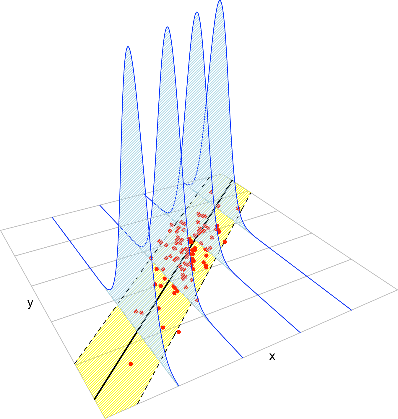
$The key concepts of the simple linear model. The red points represent a sample with population regression line $y=\beta_0+\beta_1x$ given by the black line. The yellow band denotes where $95\%$ of the data is, according to the model. The blue densities represent the conditional density of $Y$ given $X=x,$ whose means lie in the regression line.$

Figure 2.8: The key concepts of the simple linear model. The red points represent a sample with population regression line $y=\beta_0+\beta_1x$ given by the black line. The yellow band denotes where $95\%$ of the data is, according to the model. The blue densities represent the conditional density of $Y$ given $X=x,$ whose means lie in the regression line.

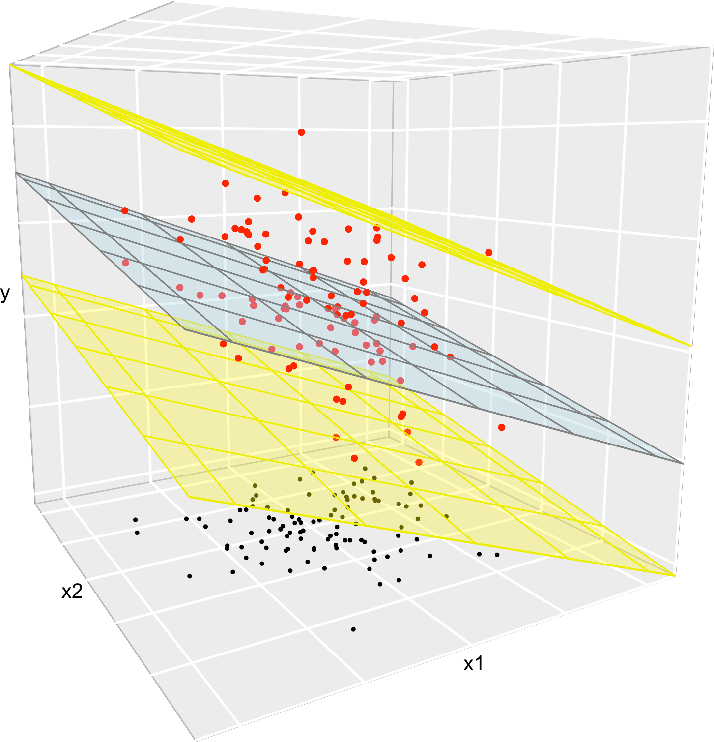
$The key concepts of the multiple linear model when $p=2.$ The red points represent a sample with population regression plane $y=\beta_0+\beta_1x_1+\beta_2x_2$ given by the blue plane. The black points represent the associated observations of the predictors. The space between the yellow planes denotes where $95\%$ of the data is, according to the model.$

Figure 2.9: The key concepts of the multiple linear model when $p=2.$ The red points represent a sample with population regression plane $y=\beta_0+\beta_1x_1+\beta_2x_2$ given by the blue plane. The black points represent the associated observations of the predictors. The space between the yellow planes denotes where $95\%$ of the data is, according to the model.

Figure 2.12 represents situations where the assumptions of the model are respected and violated, for the situation with two predictors. Clearly, the inspection of the scatterplots for identifying strange patterns is more complicated than in simple linear regression – and here we are dealing only with two predictors.

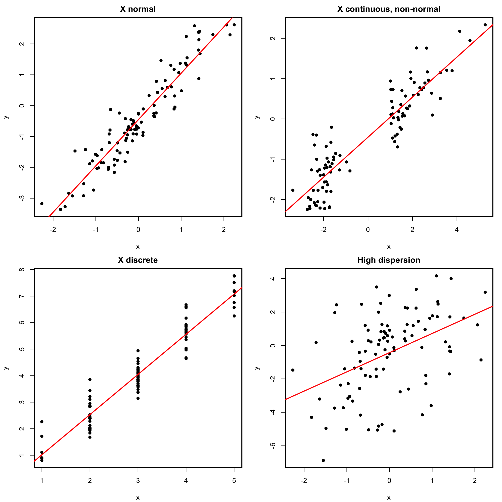
Figure 2.10: Perfectly valid simple linear models (all the assumptions are verified).

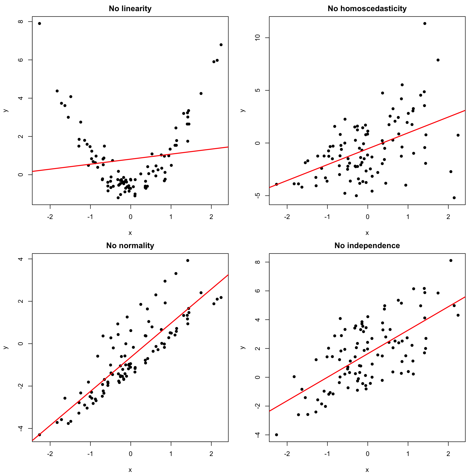
Figure 2.11: Problematic simple linear models (a single assumption does not hold).

Figure 2.12: Valid (all the assumptions are verified) and problematic (a single assumption does not hold) multiple linear models, when there are two predictors. Application available here.

The dataset assumptions.RData contains the variables x1, …, x9 and y1, …, y9. For each regression y1 ~ x1, …, y9 ~ x9:

Check whether the assumptions of the linear model are being satisfied (make a scatterplot with a regression line).
State which assumption(s) are violated and justify your answer.

After all, we already have a neat way of estimating $\boldsymbol{\beta}$ from the data… Isn’t it all is needed?↩︎