3.1 Case study: Housing values in Boston

This case study is motivated by Harrison and Rubinfeld (1978), who proposed an hedonic model⁵⁰ for determining the willingness of house buyers to pay for clean air. The study of Harrison and Rubinfeld (1978) employed data from the Boston metropolitan area, containing 560 suburbs and 14 variables. The Boston dataset is available through the file Boston.xlsx file and through the dataset MASS::Boston.

The description of the related variables can be found in ?Boston and Harrison and Rubinfeld (1978)⁵¹, but we summarize here the most important ones as they appear in Boston. They are aggregated into five categories:

• Dependent variable: medv, the median value of owner-occupied homes (in thousands of dollars).
• Structural variables indicating the house characteristics: rm (average number of rooms “in owner units”) and age (proportion of owner-occupied units built prior to 1940).
• Neighborhood variables: crim (crime rate), zn (proportion of residential areas), indus (proportion of non-retail business area), chas (whether there is river limitation), tax (cost of public services in each community), ptratio (pupil-teacher ratio), black (variable \(1000(B - 0.63)^2,\) where \(B\) is the proportion of black population – low and high values of \(B\) increase housing prices) and lstat (percent of lower status of the population).
• Accessibility variables: dis (distances to five employment centers) and rad (accessibility to radial highways – larger index denotes better accessibility).
• Air pollution variable: nox, the annual concentration of nitrogen oxide (in parts per ten million).

We begin by importing the data:

# Read data
Boston <- readxl::read_excel(path = "Boston.xlsx", sheet = 1, col_names = TRUE)

# # Alternatively
# data(Boston, package = "MASS")

A quick summary of the data is shown below:

summary(Boston)
##       crim                zn             indus            chas              nox               rm       
##  Min.   : 0.00632   Min.   :  0.00   Min.   : 0.46   Min.   :0.00000   Min.   :0.3850   Min.   :3.561  
##  1st Qu.: 0.08205   1st Qu.:  0.00   1st Qu.: 5.19   1st Qu.:0.00000   1st Qu.:0.4490   1st Qu.:5.886  
##  Median : 0.25651   Median :  0.00   Median : 9.69   Median :0.00000   Median :0.5380   Median :6.208  
##  Mean   : 3.61352   Mean   : 11.36   Mean   :11.14   Mean   :0.06917   Mean   :0.5547   Mean   :6.285  
##  3rd Qu.: 3.67708   3rd Qu.: 12.50   3rd Qu.:18.10   3rd Qu.:0.00000   3rd Qu.:0.6240   3rd Qu.:6.623  
##  Max.   :88.97620   Max.   :100.00   Max.   :27.74   Max.   :1.00000   Max.   :0.8710   Max.   :8.780  
##       age              dis              rad              tax           ptratio          black            lstat      
##  Min.   :  2.90   Min.   : 1.130   Min.   : 1.000   Min.   :187.0   Min.   :12.60   Min.   :  0.32   Min.   : 1.73  
##  1st Qu.: 45.02   1st Qu.: 2.100   1st Qu.: 4.000   1st Qu.:279.0   1st Qu.:17.40   1st Qu.:375.38   1st Qu.: 6.95  
##  Median : 77.50   Median : 3.207   Median : 5.000   Median :330.0   Median :19.05   Median :391.44   Median :11.36  
##  Mean   : 68.57   Mean   : 3.795   Mean   : 9.549   Mean   :408.2   Mean   :18.46   Mean   :356.67   Mean   :12.65  
##  3rd Qu.: 94.08   3rd Qu.: 5.188   3rd Qu.:24.000   3rd Qu.:666.0   3rd Qu.:20.20   3rd Qu.:396.23   3rd Qu.:16.95  
##  Max.   :100.00   Max.   :12.127   Max.   :24.000   Max.   :711.0   Max.   :22.00   Max.   :396.90   Max.   :37.97  
##       medv      
##  Min.   : 5.00  
##  1st Qu.:17.02  
##  Median :21.20  
##  Mean   :22.53  
##  3rd Qu.:25.00  
##  Max.   :50.00

The two goals of this case study are:

• Q1. Quantify the influence of the predictor variables in the housing prices.
• Q2. Obtain the “best possible” model for decomposing the housing prices and interpret it.

We begin by making an exploratory analysis of the data with a matrix scatterplot. Since the number of variables is high, we opt to plot only five variables: crim, dis, medv, nox, and rm. Each of them represents the five categories in which variables were classified.

car::scatterplotMatrix(~ crim + dis + medv + nox + rm, regLine = list(col = 2),
                       col = 1, smooth = list(col.smooth = 4, col.spread = 4),
                       data = Boston)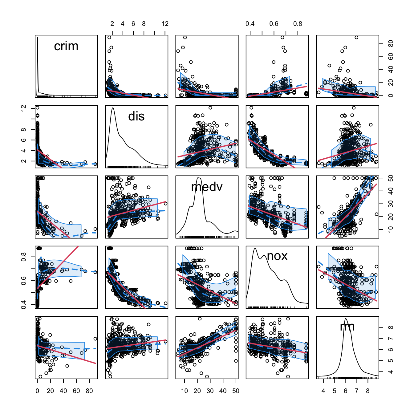

Figure 3.1: Scatterplot matrix for crim, dis, medv, nox, and rm from the Boston dataset. The diagonal panels show an estimate of the unknown pdf of each variable (see Section 6.1.2). The red and blue lines are linear and nonparametric (see Section 6.2) estimates of the regression functions for pairwise relations.

Note the peculiar distribution of crim, very concentrated at zero, and the asymmetry in medv, with a second mode associated to the most expensive properties. Inspecting the individual panels, it is clear that some nonlinearity exists in the data and that some predictors are going to be more important than others (and recall that we have plotted just a subset of all the predictors).

References

Harrison, D., and D. L. Rubinfeld. 1978. “Hedonic Housing Prices and the Demand for Clean Air.” Journal of Environmental Economics and Management 5 (1): 81–102. https://doi.org/10.1016/0095-0696(78)90006-2.

---

50. An hedonic model is a model that decomposes the price of an item into separate components that determine its price. For example, an hedonic model for the price of a house may decompose its price into the house characteristics, the kind of neighborhood, and the location.↩︎

51. But be aware of the changes in units for medv, black, lstat, and nox.↩︎