2.6 ANOVA

The variance of the error, $\sigma^2,$ plays a fundamental role in the inference for the model coefficients and in prediction. In this section we will see how the variance of $Y$ is decomposed into two parts, each corresponding to the regression and to the error, respectively. This decomposition is called the ANalysis Of VAriance (ANOVA).

An important fact to highlight prior to introducing the ANOVA decomposition is that $\bar Y=\bar{\hat{Y}}.$ ³⁸ The ANOVA decomposition considers the following measures of variation related with the response:

$\text{SST}:=\sum_{i=1}^n\big(Y_i-\bar Y\big)^2,$ the Total Sum of Squares. This is the total variation of $Y_1,\ldots,Y_n,$ since $\text{SST}=ns_y^2,$ where $s_y^2$ is the sample variance of $Y_1,\ldots,Y_n.$
$\text{SSR}:=\sum_{i=1}^n\big(\hat Y_i-\bar Y\big)^2,$ the Regression Sum of Squares. This is the variation explained by the regression plane, that is, the variation from $\bar Y$ that is explained by the estimated conditional mean $\hat Y_i=\hat\beta_0+\hat\beta_1X_{i1}+\cdots+\hat\beta_pX_{ip}$ . Also, $\text{SSR}=ns_{\hat y}^2,$ where $s_{\hat y}^2$ is the sample variance of $\hat Y_1,\ldots,\hat Y_n.$
$\text{SSE}:=\sum_{i=1}^n\big(Y_i-\hat Y_i\big)^2,$ the Sum of Squared Errors.³⁹ Is the variation around the conditional mean. Recall that $\text{SSE}=\sum_{i=1}^n \hat\varepsilon_i^2=(n-p-1)\hat\sigma^2,$ where $\hat\sigma^2$ is the rescaled sample variance of $\hat \varepsilon_1,\ldots,\hat \varepsilon_n.$

The ANOVA decomposition states that:

$\begin{align} \underbrace{\text{SST}}_{\text{Variation of }Y_i's} = \underbrace{\text{SSR}}_{\text{Variation of }\hat Y_i's} + \underbrace{\text{SSE}}_{\text{Variation of }\hat \varepsilon_i's} \tag{2.20} \end{align}$

or, equivalently (dividing by $n$ in (2.20)),

$\begin{align*} \underbrace{s_y^2}_{\text{Variance of }Y_i's} = \underbrace{s_{\hat y}^2}_{\text{Variance of }\hat Y_i's} + \underbrace{(n-p-1)/n\times\hat\sigma^2}_{\text{Variance of }\hat\varepsilon_i's}. \end{align*}$

The graphical interpretation of (2.20) when $p=1$ is shown in Figure 2.16. Figure 2.17 dynamically shows how the ANOVA decomposition places more weight on SSR or SSE according to $\hat\sigma^2$ (which is obviously driven by the value of $\sigma^2$ ).

The ANOVA table summarizes the decomposition of the variance:

	Degrees of freedom	Sum Squares	Mean Squares	$F$ -value	$p$ -value
Predictors	$p$	SSR	$\frac{\text{SSR}}{p}$	$\frac{\text{SSR}/p}{\text{SSE}/(n-p-1)}$	$p$ -value
Residuals	$n-p-1$	SSE	$\frac{\text{SSE}}{n-p-1}$

The $F$ -value of the ANOVA table represents the value of the $F$ -statistic $\frac{\text{SSR}/p}{\text{SSE}/(n-p-1)}.$ This statistic is employed to test

$\begin{align*} H_0:\beta_1=\cdots=\beta_p=0\quad\text{vs.}\quad H_1:\beta_j\neq 0\text{ for any }j\geq 1, \end{align*}$

that is, the hypothesis of no linear dependence of $Y$ on $X_1,\ldots,X_p.$ ⁴⁰ This is the so-called $F$ -test and, if $H_0$ is rejected, allows to conclude that at least one $\beta_j$ is significantly different from zero.⁴¹ It happens that

$\begin{align*} F=\frac{\text{SSR}/p}{\text{SSE}/(n-p-1)}\stackrel{H_0}{\sim} F_{p,n-p-1}, \end{align*}$

where $F_{p,n-p-1}$ represents the Snedecor’s $F$ distribution with $p$ and $n-p-1$ degrees of freedom. If $H_0$ is true, then $F$ is expected to be small since SSR will be close to zero.⁴² The $F$ -test rejects at significance level $\alpha$ for large values of the $F$ -statistic, precisely for those above the $\alpha$ -upper quantile of the $F_{p,n-p-1}$ distribution, denoted by $F_{p,n-p-1;\alpha}.$ ⁴³ That is, $H_0$ is rejected if $F>F_{p,n-p-1;\alpha}.$

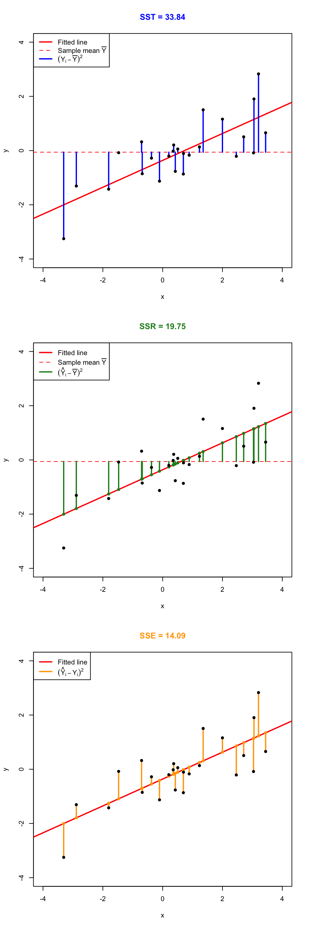
$Visualization of the ANOVA decomposition. SST measures the variation of $Y_1,\ldots,Y_n$ with respect to $\bar Y.$ SSR measures the variation of $\hat Y_1,\ldots,\hat Y_n$ with respect to $\bar{\hat Y} = \bar Y.$ SSE collects the variation between $Y_1,\ldots,Y_n$ and $\hat Y_1,\ldots,\hat Y_n,$ that is, the variation of the residuals.$

Figure 2.16: Visualization of the ANOVA decomposition. SST measures the variation of $Y_1,\ldots,Y_n$ with respect to $\bar Y.$ SSR measures the variation of $\hat Y_1,\ldots,\hat Y_n$ with respect to $\bar{\hat Y} = \bar Y.$ SSE collects the variation between $Y_1,\ldots,Y_n$ and $\hat Y_1,\ldots,\hat Y_n,$ that is, the variation of the residuals.

Figure 2.17: Illustration of the ANOVA decomposition and its dependence on $\sigma^2$ and $\hat\sigma^2.$ Larger (respectively, smaller) $\hat\sigma^2$ results in more weight placed on the SSE (SSR) term. Application available here.

The “ANOVA table” is a broad concept in statistics, with different variants. Here we are only covering the basic ANOVA table from the relation $\text{SST} = \text{SSR} + \text{SSE}.$ However, further sophistication is possible when $\text{SSR}$ is decomposed into the variations contributed by each predictor. In particular, for multiple linear regression R’s anova implements a sequential (type I) ANOVA table, which is not the previous table!

The anova function takes a model as an input and returns the following sequential ANOVA table:⁴⁴

	Degrees of freedom	Sum Squares	Mean Squares	$F$ -value	$p$ -value
Predictor 1	$1$	SSR $_1$	$\frac{\text{SSR}_1}{1}$	$\frac{\text{SSR}_1/1}{\text{SSE}/(n-p-1)}$	$p_1$
Predictor 2	$1$	SSR $_2$	$\frac{\text{SSR}_2}{1}$	$\frac{\text{SSR}_2/1}{\text{SSE}/(n-p-1)}$	$p_2$
$\vdots$	$\vdots$	$\vdots$	$\vdots$	$\vdots$	$\vdots$
Predictor $p$	$1$	SSR $_p$	$\frac{\text{SSR}_p}{1}$	$\frac{\text{SSR}_p/1}{\text{SSE}/(n-p-1)}$	$p_p$
Residuals	$n - p - 1$	SSE	$\frac{\text{SSE}}{n-p-1}$

Here the SSR $_j$ represents the regression sum of squares associated to the inclusion of $X_j$ in the model with predictors $X_1,\ldots,X_{j-1},$ this is:

$\begin{align*} \text{SSR}_j=\text{SSR}(X_1,\ldots,X_j)-\text{SSR}(X_1,\ldots,X_{j-1}). \end{align*}$

The $p$ -values $p_1,\ldots,p_p$ correspond to the testing of the hypotheses

$\begin{align*} H_0:\beta_j=0\quad\text{vs.}\quad H_1:\beta_j\neq 0, \end{align*}$

carried out inside the linear model $Y=\beta_0+\beta_1X_1+\cdots+\beta_jX_j+\varepsilon.$ This is like the $t$ -test for $\beta_j$ for the model with predictors $X_1,\ldots,X_j.$ Recall that there is no $F$ -test in this version of the ANOVA table.

In order to exactly⁴⁵ compute the simplified ANOVA table seen before, we can rely on the following ad-hoc function. The function takes as input a fitted lm:

# This function computes the simplified anova from a linear model
simpleAnova <- function(object, ...) {

  # Compute anova table
  tab <- anova(object, ...)

  # Obtain number of predictors
  p <- nrow(tab) - 1

  # Add predictors row
  predictorsRow <- colSums(tab[1:p, 1:2])
  predictorsRow <- c(predictorsRow, predictorsRow[2] / predictorsRow[1])

  # F-quantities
  Fval <- predictorsRow[3] / tab[p + 1, 3]
  pval <- pf(Fval, df1 = p, df2 = tab$Df[p + 1], lower.tail = FALSE)
  predictorsRow <- c(predictorsRow, Fval, pval)

  # Simplified table
  tab <- rbind(predictorsRow, tab[p + 1, ])
  row.names(tab)[1] <- "Predictors"
  return(tab)

}

2.6.1 Case study application

Let’s compute the ANOVA decomposition of modWine1 and modWine2 to test the existence of linear dependence.

# Models
modWine1 <- lm(Price ~ ., data = wine)
modWine2 <- lm(Price ~ . - FrancePop, data = wine)

# Simplified table
simpleAnova(modWine1)
## Analysis of Variance Table
## 
## Response: Price
##            Df Sum Sq Mean Sq F value    Pr(>F)    
## Predictors  5 8.6671 1.73343  20.188 2.232e-07 ***
## Residuals  21 1.8032 0.08587                      
## ---
## Signif. codes:  0 '***' 0.001 '**' 0.01 '*' 0.05 '.' 0.1 ' ' 1
simpleAnova(modWine2)
## Analysis of Variance Table
## 
## Response: Price
##            Df Sum Sq Mean Sq F value    Pr(>F)    
## Predictors  4 8.6645 2.16613   26.39 4.057e-08 ***
## Residuals  22 1.8058 0.08208                      
## ---
## Signif. codes:  0 '***' 0.001 '**' 0.01 '*' 0.05 '.' 0.1 ' ' 1
# The null hypothesis of no linear dependence is emphatically rejected in
# both models

# R's ANOVA table -- warning this is not what we saw in lessons
anova(modWine1)
## Analysis of Variance Table
## 
## Response: Price
##             Df Sum Sq Mean Sq F value    Pr(>F)    
## WinterRain   1 0.1905  0.1905  2.2184 0.1512427    
## AGST         1 5.8989  5.8989 68.6990 4.645e-08 ***
## HarvestRain  1 1.6662  1.6662 19.4051 0.0002466 ***
## Age          1 0.9089  0.9089 10.5852 0.0038004 ** 
## FrancePop    1 0.0026  0.0026  0.0305 0.8631279    
## Residuals   21 1.8032  0.0859                      
## ---
## Signif. codes:  0 '***' 0.001 '**' 0.01 '*' 0.05 '.' 0.1 ' ' 1

Compute the ANOVA table for the regression Price ~ WinterRain + AGST + HarvestRain + Age in the wine dataset. Check that the $p$ -value for the $F$ -test given in summary and by simpleAnova are the same.

For the y6 ~ x6 and y7 ~ x7 in the assumptions dataset, compute their ANOVA tables. Check that the $p$ -values of the $t$ -test for $\beta_1$ and the $F$ -test are the same (any explanation of why this is so?).

This is an important result that can be checked using the matrix notation introduced in Section 2.2.3.↩︎
Recall that SSE and RSS (of the least squares estimator $\hat{\boldsymbol{\beta}}$ ) are two names for the same quantity (that appears in different contexts): $\text{SSE}=\sum_{i=1}^n\big(Y_i-\hat Y_i\big)^2=\sum_{i=1}^n\big(Y_i-\hat \beta_0-\hat \beta_1X_{i1}-\cdots-\hat \beta_pX_{ip}\big)^2=\mathrm{RSS}(\hat{\boldsymbol{\beta}}).$ ↩︎
Geometrically: the plane is completely flat, it does not have any inclination in the $Y$ direction.↩︎
And therefore, there is a statistical meaningful (i.e., not constant) linear trend to model.↩︎
Little variation is explained by the regression model since $\hat{\boldsymbol{\beta}}\approx\mathbf{0}.$ ↩︎
In R, qf(p = 1 - alpha, df1 = n - p - 1, df2 = p) or qf(p = alpha, df1 = n - p - 1, df2 = p, lower.tail = FALSE).↩︎
More complex – included here just for clarification of the anova’s output.↩︎
Note that, if mod <- lm(resp ~ preds, data) represents a model with response resp and predictors preds, and mod0, is the intercept-only model mod0 <- lm(resp ~ 1, data) that does not contain predictors, anova(mod0, mod) gives a similar, output to the seen ANOVA table. Precisely, the first row of the outputted table stands for the SST and the second row for the SSE row (so we call it the SST–SSE table). The SSR row is not present. The seen ANOVA table (which contains SSR and SSE) and the SST–SSE table encode the same information due to the ANOVA decomposition. So it is a matter of taste and tradition to employ one or the other. In particular, both have the $F$ -test and its associated $p$ -value (in the SSE row for the SST–SSE table).↩︎