A.4 Dealing with missing data
Missing data, codified as NA in R, can be problematic in predictive modeling. By default, most of the regression models in R work with the complete cases of the data, that is, they exclude the cases in which there is at least one NA. This may be problematic in certain circumstances. Let’s see an example.
# The airquality dataset contains NA's
data(airquality)
head(airquality)
##   Ozone Solar.R Wind Temp Month Day
## 1    41     190  7.4   67     5   1
## 2    36     118  8.0   72     5   2
## 3    12     149 12.6   74     5   3
## 4    18     313 11.5   62     5   4
## 5    NA      NA 14.3   56     5   5
## 6    28      NA 14.9   66     5   6
summary(airquality)
##      Ozone           Solar.R           Wind             Temp           Month            Day
##  Min.   :  1.00   Min.   :  7.0   Min.   : 1.700   Min.   :56.00   Min.   :5.000   Min.   : 1.0
##  1st Qu.: 18.00   1st Qu.:115.8   1st Qu.: 7.400   1st Qu.:72.00   1st Qu.:6.000   1st Qu.: 8.0
##  Median : 31.50   Median :205.0   Median : 9.700   Median :79.00   Median :7.000   Median :16.0
##  Mean   : 42.13   Mean   :185.9   Mean   : 9.958   Mean   :77.88   Mean   :6.993   Mean   :15.8
##  3rd Qu.: 63.25   3rd Qu.:258.8   3rd Qu.:11.500   3rd Qu.:85.00   3rd Qu.:8.000   3rd Qu.:23.0
##  Max.   :168.00   Max.   :334.0   Max.   :20.700   Max.   :97.00   Max.   :9.000   Max.   :31.0
##  NA's   :37       NA's   :7

# Let's add more NA's for the sake of illustration
set.seed(123456)
airquality$Solar.R[runif(nrow(airquality)) < 0.7] <- NA
airquality$Day[runif(nrow(airquality)) < 0.1] <- NA

# See what are the fully-observed cases
comp <- complete.cases(airquality)
mean(comp) # Only 15% of cases are fully observed
## [1] 0.1568627

# Complete cases
head(airquality[comp, ])
##    Ozone Solar.R Wind Temp Month Day
## 1     41     190  7.4   67     5   1
## 2     36     118  8.0   72     5   2
## 9      8      19 20.1   61     5   9
## 13    11     290  9.2   66     5  13
## 14    14     274 10.9   68     5  14
## 15    18      65 13.2   58     5  15

# Linear model on all the variables
summary(lm(Ozone ~ ., data = airquality)) # 129 not included
##
## Call:
## lm(formula = Ozone ~ ., data = airquality)
##
## Residuals:
##     Min      1Q  Median      3Q     Max
## -23.790 -10.910  -2.249  10.960  33.246
##
## Coefficients:
##              Estimate Std. Error t value Pr(>|t|)
## (Intercept) -71.50880   31.49703  -2.270 0.035704 *
## Solar.R      -0.01112    0.03376  -0.329 0.745596
## Wind         -0.61129    0.96113  -0.636 0.532769
## Temp          1.82870    0.42224   4.331 0.000403 ***
## Month        -2.86513    2.22222  -1.289 0.213614
## Day          -0.28710    0.41700  -0.688 0.499926
## ---
## Signif. codes:  0 '***' 0.001 '**' 0.01 '*' 0.05 '.' 0.1 ' ' 1
##
## Residual standard error: 16.12 on 18 degrees of freedom
##   (129 observations deleted due to missingness)
## Multiple R-squared:  0.5957, Adjusted R-squared:  0.4833
## F-statistic: 5.303 on 5 and 18 DF,  p-value: 0.00362

# Caution! Even if the problematic variable is excluded, only
# the complete observations are employed
summary(lm(Ozone ~ . - Solar.R, data = airquality))
##
## Call:
## lm(formula = Ozone ~ . - Solar.R, data = airquality)
##
## Residuals:
##    Min     1Q Median     3Q    Max
## -24.43 -11.56  -1.67  11.19  33.11
##
## Coefficients:
##             Estimate Std. Error t value Pr(>|t|)
## (Intercept) -72.2501    30.6707  -2.356 0.029386 *
## Wind         -0.6236     0.9376  -0.665 0.514001
## Temp          1.7980     0.4021   4.472 0.000261 ***
## Month        -2.6533     2.0767  -1.278 0.216762
## Day          -0.2944     0.4065  -0.724 0.477851
## ---
## Signif. codes:  0 '***' 0.001 '**' 0.01 '*' 0.05 '.' 0.1 ' ' 1
##
## Residual standard error: 15.74 on 19 degrees of freedom
##   (129 observations deleted due to missingness)
## Multiple R-squared:  0.5932, Adjusted R-squared:  0.5076
## F-statistic: 6.927 on 4 and 19 DF,  p-value: 0.001291

# Notice the difference with
summary(lm(Ozone ~ ., data = subset(airquality, select = -Solar.R)))
##
## Call:
## lm(formula = Ozone ~ ., data = subset(airquality, select = -Solar.R))
##
## Residuals:
##     Min      1Q  Median      3Q     Max
## -42.677 -12.609  -3.125  11.993  98.805
##
## Coefficients:
##             Estimate Std. Error t value Pr(>|t|)
## (Intercept) -74.4456    25.8567  -2.879  0.00488 **
## Wind         -3.1064     0.7028  -4.420 2.51e-05 ***
## Temp          2.1666     0.2876   7.534 2.25e-11 ***
## Month        -3.6493     1.6343  -2.233  0.02778 *
## Day           0.3162     0.2549   1.241  0.21768
## ---
## Signif. codes:  0 '***' 0.001 '**' 0.01 '*' 0.05 '.' 0.1 ' ' 1
##
## Residual standard error: 22.12 on 100 degrees of freedom
##   (48 observations deleted due to missingness)
## Multiple R-squared:  0.5963, Adjusted R-squared:  0.5801
## F-statistic: 36.92 on 4 and 100 DF,  p-value: < 2.2e-16

# Model selection can be problematic with missing data, since
# the number of complete cases changes with the addition or
# removing of predictors
mod <- lm(Ozone ~ ., data = airquality)

# stepAIC drops an error
modAIC <- MASS::stepAIC(mod)
## Start:  AIC=138.55
## Ozone ~ Solar.R + Wind + Temp + Month + Day
##
##           Df Sum of Sq    RSS    AIC
## - Solar.R  1      28.2 4708.1 136.70
## - Wind     1     105.2 4785.0 137.09
## - Day      1     123.2 4803.1 137.18
## <none>                 4679.9 138.55
## - Month    1     432.2 5112.1 138.67
## - Temp     1    4876.6 9556.5 153.69
## Error in MASS::stepAIC(mod): number of rows in use has changed: remove missing values?

# Also, this will be problematic (the number of complete
# cases changes with the predictors considered!)
modBIC <- MASS::stepAIC(mod, k = log(nrow(airquality)))
## Start:  AIC=156.73
## Ozone ~ Solar.R + Wind + Temp + Month + Day
##
##           Df Sum of Sq    RSS    AIC
## - Solar.R  1      28.2 4708.1 151.85
## - Wind     1     105.2 4785.0 152.24
## - Day      1     123.2 4803.1 152.33
## - Month    1     432.2 5112.1 153.82
## <none>                 4679.9 156.73
## - Temp     1    4876.6 9556.5 168.84
## Error in MASS::stepAIC(mod, k = log(nrow(airquality))): number of rows in use has changed: remove missing values?

# Comparison of AICs or BICs is spurious: the scale of the
# likelihood changes with the sample size (the likelihood
# decreases with n), which increases AIC / BIC with n.
# Hence using BIC / AIC is not adequate for model selection
# with missing data.
AIC(lm(Ozone ~ ., data = airquality))
## [1] 208.6604
AIC(lm(Ozone ~ ., data = subset(airquality, select = -Solar.R)))
## [1] 955.0681

# Considers only complete cases including Solar.R
AIC(lm(Ozone ~ . - Solar.R, data = airquality))
## [1] 206.8047
We have seen the problems that missing data may cause in regression models. There are many techniques designed to handle missing data, depending on the missing data mechanism (whether is it completely at random or whether there is some pattern in the missing process) and the approach to impute the data (parametric, nonparametric, Bayesian, etc). We do not give an exhaustive view of the topic here, but we outline three concrete approaches to handle missing data in practice:
- Use complete cases. This is the simplest solution and can be achieved by restricting the analysis to the set of fully-observed observations. The advantage of this solution is that it can be implemented very easily by using the
complete.casesorna.excludefunctions. However, an undesirable consequence is that we may lose a substantial amount of data and therefore the precision of the estimators will be lower. In addition, it may lead to a biased representation of the original data (if the missing process is associated with the values of the response or predictors). - Remove predictors with many missing data. This is another simple solution that is useful in case most of the missing data is concentrated in one predictor.
- Use imputation for the missing values. The idea is to replace the missing observations on the response or the predictors with artificial values that try to preserve the dataset structure:
- When the response is missing, we can use a predictive model to predict the missing response, then create a new fully-observed dataset containing the predictions instead of the missing values, and finally re-estimate the predictive model in this expanded dataset. This approach is attractive if most of the missing data is in the response.
- When different predictors and the response are missing, we can use a direct imputation for them. The simplest approach is to replace the missing data with the sample mean of the observed cases (in the case of quantitative variables). Another approach is to input sample means for the predictors, then use the reconstructed dataset to predict the missing responses. These and more sophisticated imputation methods, based on predictive models, are available within the
micepackage.248 This approach is interesting if the data contains manyNAs scattered in different predictors (hence a complete-cases analysis will be inefficient).
Let’s put in practice these three approaches in the previous example.
# The complete cases approach is the default in R
summary(lm(Ozone ~ ., data = airquality))
##
## Call:
## lm(formula = Ozone ~ ., data = airquality)
##
## Residuals:
##     Min      1Q  Median      3Q     Max
## -23.790 -10.910  -2.249  10.960  33.246
##
## Coefficients:
##              Estimate Std. Error t value Pr(>|t|)
## (Intercept) -71.50880   31.49703  -2.270 0.035704 *
## Solar.R      -0.01112    0.03376  -0.329 0.745596
## Wind         -0.61129    0.96113  -0.636 0.532769
## Temp          1.82870    0.42224   4.331 0.000403 ***
## Month        -2.86513    2.22222  -1.289 0.213614
## Day          -0.28710    0.41700  -0.688 0.499926
## ---
## Signif. codes:  0 '***' 0.001 '**' 0.01 '*' 0.05 '.' 0.1 ' ' 1
##
## Residual standard error: 16.12 on 18 degrees of freedom
##   (129 observations deleted due to missingness)
## Multiple R-squared:  0.5957, Adjusted R-squared:  0.4833
## F-statistic: 5.303 on 5 and 18 DF,  p-value: 0.00362

# However, since the complete cases that R is going to consider
# depends on which predictors are included, it is safer to
# exclude NA's explicitly before the fitting of a model.
airqualityNoNA <- na.exclude(airquality)
summary(airqualityNoNA)
##      Ozone          Solar.R           Wind             Temp           Month           Day
##  Min.   : 8.00   Min.   : 13.0   Min.   : 6.300   Min.   :58.00   Min.   :5.00   Min.   : 1.00
##  1st Qu.:13.00   1st Qu.: 61.5   1st Qu.: 9.575   1st Qu.:65.50   1st Qu.:5.00   1st Qu.:11.25
##  Median :17.00   Median :178.5   Median :11.500   Median :71.50   Median :6.00   Median :16.50
##  Mean   :28.21   Mean   :161.8   Mean   :11.887   Mean   :72.54   Mean   :6.75   Mean   :15.79
##  3rd Qu.:36.25   3rd Qu.:255.0   3rd Qu.:14.300   3rd Qu.:79.50   3rd Qu.:9.00   3rd Qu.:20.25
##  Max.   :96.00   Max.   :334.0   Max.   :20.700   Max.   :97.00   Max.   :9.00   Max.   :29.00

# The package VIM has a function to visualize where the missing
# data is present. It gives the percentage of NA's for each
# variable and for the most important combinations of NA's.
VIM::aggr(airquality)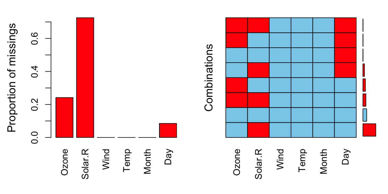
# Stepwise regression without NA's -- no problem
modBIC1 <- MASS::stepAIC(lm(Ozone ~ ., data = airqualityNoNA),
                         k = log(nrow(airqualityNoNA)), trace = 0)
summary(modBIC1)
##
## Call:
## lm(formula = Ozone ~ Temp, data = airqualityNoNA)
##
## Residuals:
##     Min      1Q  Median      3Q     Max
## -27.645 -13.180  -0.136   8.926  37.666
##
## Coefficients:
##             Estimate Std. Error t value Pr(>|t|)
## (Intercept) -90.1846    24.6414  -3.660  0.00138 **
## Temp          1.6321     0.3367   4.847 7.63e-05 ***
## ---
## Signif. codes:  0 '***' 0.001 '**' 0.01 '*' 0.05 '.' 0.1 ' ' 1
##
## Residual standard error: 15.95 on 22 degrees of freedom
## Multiple R-squared:  0.5164, Adjusted R-squared:  0.4944
## F-statistic: 23.49 on 1 and 22 DF,  p-value: 7.634e-05

# But we only take into account 16% of the original data
nrow(airqualityNoNA) / nrow(airquality)
## [1] 0.1568627

# Removing the predictor with many NA's, as we did before
# We also exclude NA's from other predictors
airqualityNoSolar.R <- na.exclude(subset(airquality, select = -Solar.R))
modBIC2 <- MASS::stepAIC(lm(Ozone ~ ., data = airqualityNoSolar.R),
                         k = log(nrow(airqualityNoSolar.R)), trace = 0)
summary(modBIC2)
##
## Call:
## lm(formula = Ozone ~ Wind + Temp + Month, data = airqualityNoSolar.R)
##
## Residuals:
##     Min      1Q  Median      3Q     Max
## -43.973 -14.170  -3.107  10.638 102.297
##
## Coefficients:
##             Estimate Std. Error t value Pr(>|t|)
## (Intercept) -67.7279    25.3507  -2.672   0.0088 **
## Wind         -3.0439     0.7028  -4.331 3.51e-05 ***
## Temp          2.1323     0.2870   7.429 3.59e-11 ***
## Month        -3.6167     1.6384  -2.207   0.0295 *
## ---
## Signif. codes:  0 '***' 0.001 '**' 0.01 '*' 0.05 '.' 0.1 ' ' 1
##
## Residual standard error: 22.17 on 101 degrees of freedom
## Multiple R-squared:  0.5901, Adjusted R-squared:  0.5779
## F-statistic: 48.46 on 3 and 101 DF,  p-value: < 2.2e-16
# In this example the approach works well because most of
# the NA's are associated to the variable Solar.R

# Input data using the sample mean
library(mice)
airqualityMean <- complete(mice(data = airquality, m = 1, method = "mean"))
##
##  iter imp variable
##   1   1  Ozone  Solar.R  Day
##   2   1  Ozone  Solar.R  Day
##   3   1  Ozone  Solar.R  Day
##   4   1  Ozone  Solar.R  Day
##   5   1  Ozone  Solar.R  Day
head(airqualityMean)
##      Ozone  Solar.R Wind Temp Month      Day
## 1 41.00000 190.0000  7.4   67     5  1.00000
## 2 36.00000 118.0000  8.0   72     5  2.00000
## 3 12.00000 181.7857 12.6   74     5  3.00000
## 4 18.00000 181.7857 11.5   62     5 15.62857
## 5 42.12931 181.7857 14.3   56     5  5.00000
## 6 28.00000 181.7857 14.9   66     5 15.62857
# Explanation of the syntax:
# - mice::complete() serves to retrieve the completed dataset from
#   the mids object.
# - m = 1 specifies that we only want a reconstruction of the
#   dataset because the imputation method is deterministic
#   (it could be random).
# - method = "mean" says that we want the sample mean to be
#   used to fill NA's in all the columns. This only works
#   properly for quantitative variables.

# Impute using linear regression for the response (first column)
# and mean for the predictors (remaining five columns)
airqualityLm <- complete(mice(data = airquality, m = 1,
                              method = c("norm.predict", rep("mean", 5))))
##
##  iter imp variable
##   1   1  Ozone  Solar.R  Day
##   2   1  Ozone  Solar.R  Day
##   3   1  Ozone  Solar.R  Day
##   4   1  Ozone  Solar.R  Day
##   5   1  Ozone  Solar.R  Day
head(airqualityLm)
##       Ozone  Solar.R Wind Temp Month      Day
## 1  41.00000 190.0000  7.4   67     5  1.00000
## 2  36.00000 118.0000  8.0   72     5  2.00000
## 3  12.00000 181.7857 12.6   74     5  3.00000
## 4  18.00000 181.7857 11.5   62     5 15.62857
## 5 -13.35375 181.7857 14.3   56     5  5.00000
## 6  28.00000 181.7857 14.9   66     5 15.62857

# Imputed data -- some extrapolation problems may happen
airqualityLm$Ozone[is.na(airquality$Ozone)]
##  [1] -13.3537515  33.3839709 -15.1032941  -6.4344422  15.0745276  43.7185093  34.5128480   0.1488983  57.7500138
## [10]  62.1313290  30.1891953  70.4905697  72.0216949  75.6909337  38.1841717  43.5104926  57.9764970  69.7165869
## [19]  63.0884481  51.9374205  50.0400961  56.8792515  41.2844048  49.6257521  33.0354266  67.4490679  48.9905942
## [28]  54.0457773  51.9941898  50.1697328  46.1697595  71.3235772  49.9344726  39.0222991  26.9297719  77.0827188
## [37]  26.9508942

# Notice that the imputed data is the same (except for a small
# truncation that is introduced by mice) as
predict(lm(airquality$Ozone ~ ., data = airqualityMean),
        newdata = airqualityMean[is.na(airquality$Ozone), -1])
##           5          10          25          26          27          32          33          34          35          36
## -13.3537515  33.3839709 -15.1032941  -6.4344422  15.0745276  43.7185093  34.5128480   0.1488983  57.7500138  62.1313290
##          37          39          42          43          45          46          52          53          54          55
##  30.1891953  70.4905697  72.0216949  75.6909337  38.1841717  43.5104926  57.9764970  69.7165869  63.0884481  51.9374205
##          56          57          58          59          60          61          65          72          75          83
##  50.0400961  56.8792515  41.2844048  49.6257521  33.0354266  67.4490679  48.9905942  54.0457773  51.9941898  50.1697328
##          84         102         103         107         115         119         150
##  46.1697595  71.3235772  49.9344726  39.0222991  26.9297719  77.0827188  26.9508942

# Removing the truncation with ridge = 0
complete(mice(data = airquality, m = 1,
              method = c("norm.predict", rep("mean", 5)),
              ridge = 0))[is.na(airquality$Ozone), 1]
##
##  iter imp variable
##   1   1  Ozone  Solar.R  Day
##   2   1  Ozone  Solar.R  Day
##   3   1  Ozone  Solar.R  Day
##   4   1  Ozone  Solar.R  Day
##   5   1  Ozone  Solar.R  Day
##  [1] -13.3537515  33.3839709 -15.1032941  -6.4344422  15.0745276  43.7185093  34.5128480   0.1488983  57.7500138
## [10]  62.1313290  30.1891953  70.4905697  72.0216949  75.6909337  38.1841717  43.5104926  57.9764970  69.7165869
## [19]  63.0884481  51.9374205  50.0400961  56.8792515  41.2844048  49.6257521  33.0354266  67.4490679  48.9905942
## [28]  54.0457773  51.9941898  50.1697328  46.1697595  71.3235772  49.9344726  39.0222991  26.9297719  77.0827188
## [37]  26.9508942

# The default mice's method (predictive mean matching) works
# better in this case (in the sense that it does not yield
# negative Ozone values)
# Notice that there is randomness in the imputation!
airqualityMice <- complete(mice(data = airquality, m = 1, seed = 123))
##
##  iter imp variable
##   1   1  Ozone  Solar.R  Day
##   2   1  Ozone  Solar.R  Day
##   3   1  Ozone  Solar.R  Day
##   4   1  Ozone  Solar.R  Day
##   5   1  Ozone  Solar.R  Day
head(airqualityMice)
##   Ozone Solar.R Wind Temp Month Day
## 1    41     190  7.4   67     5   1
## 2    36     118  8.0   72     5   2
## 3    12      64 12.6   74     5   3
## 4    18      44 11.5   62     5  11
## 5    19      27 14.3   56     5   5
## 6    28     286 14.9   66     5  22
Check the available methods for
mice::miceat?mice. There are specific methods for different kinds of variables (numeric, factor with two levels, factors of more than two levels) and fairly advanced imputation methods.↩︎