3.4 Nonlinear relationships

3.4.1 Transformations in the simple linear model

The linear model is termed linear not only because the form it assumes for the regression function $m$ is linear, but because the effects of the parameters are linear. Indeed, the predictor $X$ may exhibit a nonlinear effect on the response $Y$ and still be a linear model! For example, the following models can be transformed into simple linear models:

$Y=\beta_0+\beta_1X^2+\varepsilon.$
$Y=\beta_0+\beta_1\log(X)+\varepsilon.$
$Y=\beta_0+\beta_1(X^3-\log(|X|) + 2^{X})+\varepsilon.$

The trick is to work with a transformed predictor $\tilde{X}$ as a replacement of the original predictor $X.$ Then, for the above examples, rather than working with the sample $\{(X_i,Y_i)\}_{i=1}^n,$ we consider the transformed sample $\{(\tilde X_i,Y_i)\}_{i=1}^n$ with:

$\tilde X_i=X_i^2,$ $i=1,\ldots,n.$
$\tilde X_i=\log(X_i),$ $i=1,\ldots,n.$
$\tilde X_i=X_i^3-\log(|X_i|) + 2^{X_i},$ $i=1,\ldots,n.$

An example of this simple but powerful trick is given as follows. The left panel of Figure 3.6 shows the scatterplot for some data y and x, together with its fitted regression line. Clearly, the data does not follow a linear pattern, but a nonlinear one, similar to a parabola $y=x^2.$ Hence, y might be better explained by the square of x, x^2, rather than by x. Indeed, if we plot y against x^2 in the right panel of Figure 3.6, we can see that the relation of y and x^2 is now linear!

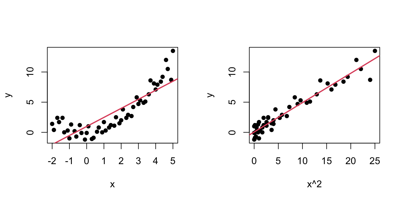
$Left: quadratic pattern when plotting $Y$ against $X.$ Right: linearized pattern when plotting $Y$ against $X^2.$ In red, the fitted regression line.$

Figure 3.6: Left: quadratic pattern when plotting $Y$ against $X.$ Right: linearized pattern when plotting $Y$ against $X^2.$ In red, the fitted regression line.

Figure 3.7: Illustration of the choice of the nonlinear transformation. Application available here.

In conclusion, with a simple trick we have drastically increased the explanation of the response. However, there is a catch: knowing which transformation is required in order to linearize the relation between response and the predictor is a kind of art which requires good eyeballing. A first approach is to try with one of the usual transformations, displayed in Figure 3.8, depending on the pattern of the data. Figure 3.7 illustrates how to choose an adequate transformation for linearizing certain nonlinear data patterns.

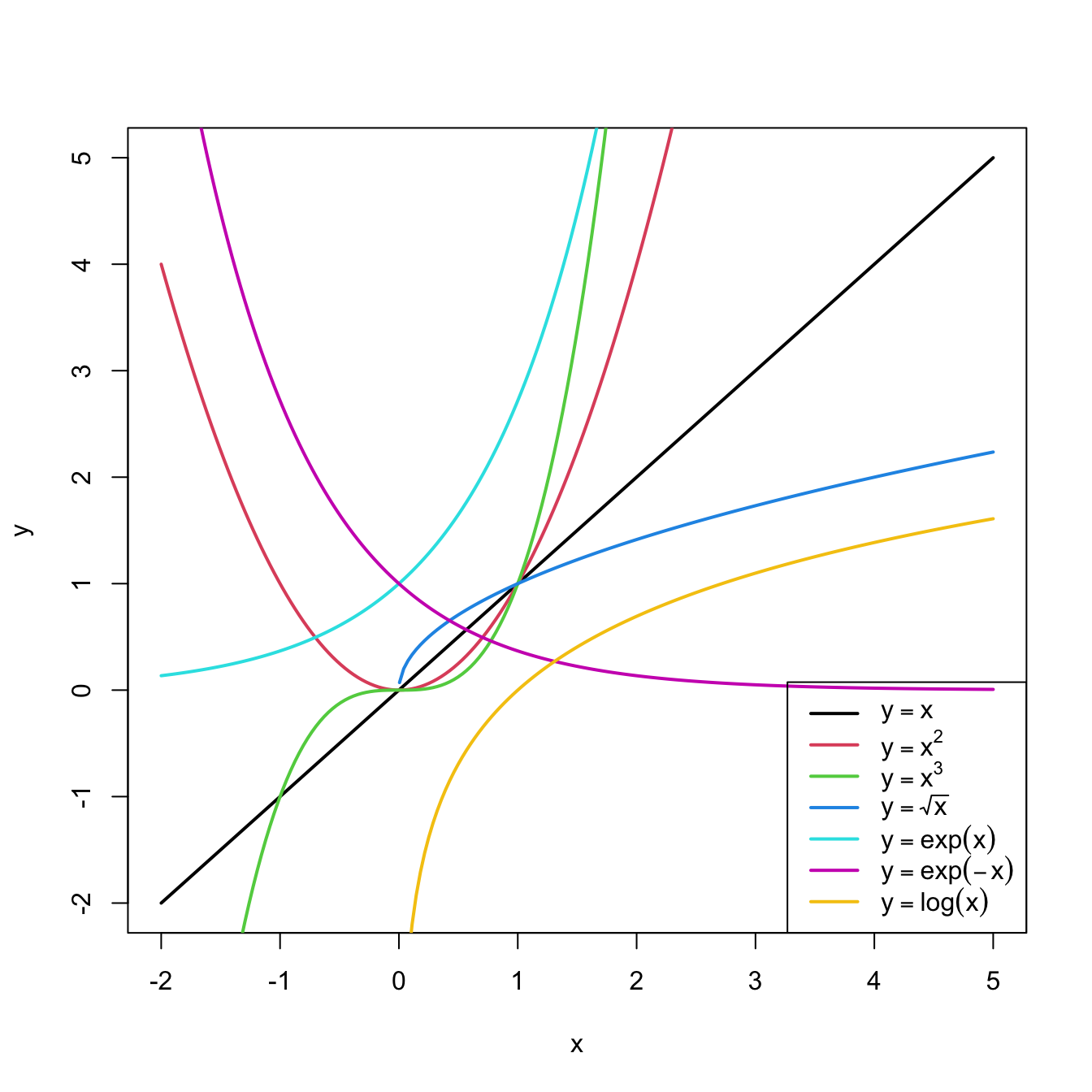
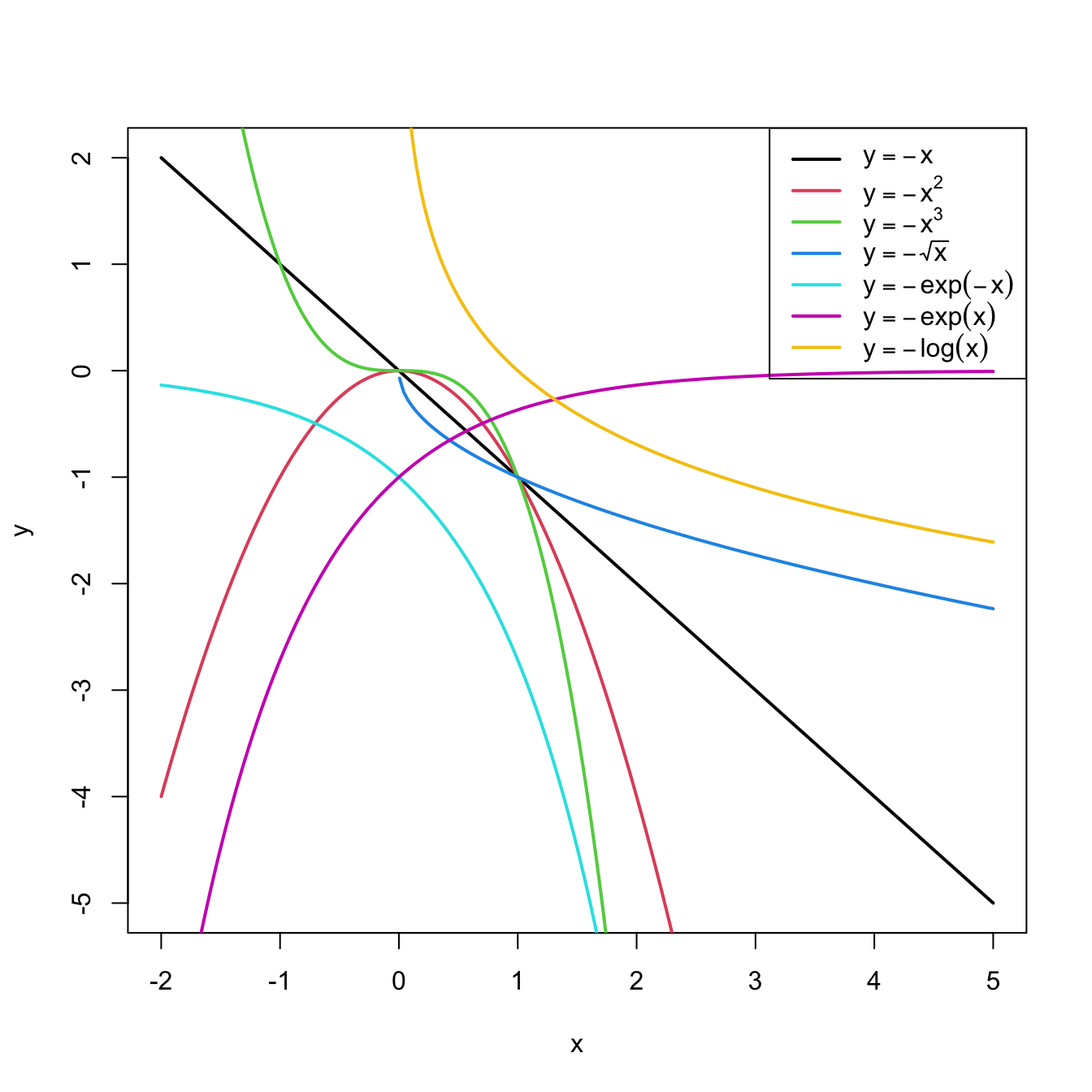
Figure 3.8: Some common nonlinear transformations and their negative counterparts. Recall the domain of definition of each transformation.

If you apply a nonlinear transformation, namely $f,$ and fit the linear model $Y=\beta_0+\beta_1 f(X)+\varepsilon,$ then there is no point in also fitting the model resulting from the negative transformation $-f.$ The model with $-f$ is exactly the same as the one with $f$ but with the sign of $\beta_1$ flipped.

As a rule of thumb, use Figure 3.8 with the transformations to compare it with the data pattern, choose the most similar curve, and apply the corresponding function with positive sign (for simpler interpretation).

Let’s see how to transform the predictor and perform the regressions behind Figure 3.6.

# Data
x <- c(-2, -1.9, -1.7, -1.6, -1.4, -1.3, -1.1, -1, -0.9, -0.7, -0.6,
       -0.4, -0.3, -0.1, 0, 0.1, 0.3, 0.4, 0.6, 0.7, 0.9, 1, 1.1, 1.3,
       1.4, 1.6, 1.7, 1.9, 2, 2.1, 2.3, 2.4, 2.6, 2.7, 2.9, 3, 3.1,
       3.3, 3.4, 3.6, 3.7, 3.9, 4, 4.1, 4.3, 4.4, 4.6, 4.7, 4.9, 5)
y <- c(1.4, 0.4, 2.4, 1.7, 2.4, 0, 0.3, -1, 1.3, 0.2, -0.7, 1.2, -0.1,
       -1.2, -0.1, 1, -1.1, -0.9, 0.1, 0.8, 0, 1.7, 0.3, 0.8, 1.2, 1.1,
       2.5, 1.5, 2, 3.8, 2.4, 2.9, 2.7, 4.2, 5.8, 4.7, 5.3, 4.9, 5.1,
       6.3, 8.6, 8.1, 7.1, 7.9, 8.4, 9.2, 12, 10.5, 8.7, 13.5)

# Data frame (a matrix with column names)
nonLinear <- data.frame(x = x, y = y)

# We create a new column inside nonLinear, called x2, that contains the
# new variable x^2
nonLinear$x2 <- nonLinear$x^2
# If you wish to remove it
# nonLinear$x2 <- NULL

# Regressions
mod1 <- lm(y ~ x, data = nonLinear)
mod2 <- lm(y ~ x2, data = nonLinear)
summary(mod1)
## 
## Call:
## lm(formula = y ~ x, data = nonLinear)
## 
## Residuals:
##     Min      1Q  Median      3Q     Max 
## -2.5268 -1.7513 -0.4017  0.9750  5.0265 
## 
## Coefficients:
##             Estimate Std. Error t value Pr(>|t|)    
## (Intercept)   0.9771     0.3506   2.787   0.0076 ** 
## x             1.4993     0.1374  10.911 1.35e-14 ***
## ---
## Signif. codes:  0 '***' 0.001 '**' 0.01 '*' 0.05 '.' 0.1 ' ' 1
## 
## Residual standard error: 2.005 on 48 degrees of freedom
## Multiple R-squared:  0.7126, Adjusted R-squared:  0.7067 
## F-statistic:   119 on 1 and 48 DF,  p-value: 1.353e-14
summary(mod2)
## 
## Call:
## lm(formula = y ~ x2, data = nonLinear)
## 
## Residuals:
##     Min      1Q  Median      3Q     Max 
## -3.0418 -0.5523 -0.1465  0.6286  1.8797 
## 
## Coefficients:
##             Estimate Std. Error t value Pr(>|t|)    
## (Intercept)  0.05891    0.18462   0.319    0.751    
## x2           0.48659    0.01891  25.725   <2e-16 ***
## ---
## Signif. codes:  0 '***' 0.001 '**' 0.01 '*' 0.05 '.' 0.1 ' ' 1
## 
## Residual standard error: 0.9728 on 48 degrees of freedom
## Multiple R-squared:  0.9324, Adjusted R-squared:  0.931 
## F-statistic: 661.8 on 1 and 48 DF,  p-value: < 2.2e-16
# mod2 has a larger R^2. Also notice the intercept is not significative

A fast way of performing and summarizing the quadratic fit is

summary(lm(y ~ I(x^2), data = nonLinear))

The I() function wrapping x^2 is fundamental when applying arithmetic operations in the predictor. The symbols +, *, ^, … have different meaning when inputted in a formula, so it is required to use I() to indicate that they must be interpreted in their arithmetic meaning and that the result of the expression denotes a new predictor. For example, use I((x - 1)^3 - log(3 * x)) to apply the transformation (x - 1)^3 - log(3 * x).

Load the dataset assumptions.RData. We are going to work with the regressions y2 ~ x2, y3 ~ x3, y8 ~ x8, and y9 ~ x9, in order to identify which transformation of Figure 3.8 gives the best fit. For these, do the following:

Find the transformation that yields the largest $R^2.$
Compare the original and transformed linear models.

Hints:

y2 ~ x2 has a negative dependence, so look at the right panel of Figure 3.7.
y3 ~ x3 seems to have just a subtle nonlinearity… Will it be worth to attempt a transformation?
For y9 ~ x9, try also with exp(-abs(x9)), log(abs(x9)), and 2^abs(x9).

The nonlinear transformations introduced for the simple linear model are readily applicable in the multiple linear model. Consequently, the multiple linear model is able to approximate regression functions with nonlinear forms, if appropriate nonlinear transformations for the predictors are used.⁶³

3.4.2 Polynomial transformations

Polynomial models are a powerful nonlinear extension of the linear model. These are constructed by replacing each predictor $X_j$ by a set of monomials $(X_j,X_j^2,\ldots,X_j^{k_j})$ constructed from $X_j.$ In the simpler case with a single predictor⁶⁴ $X,$ we have the $k$-th order polynomial fit:

\[\begin{align*} Y=\beta_0+\beta_1X+\cdots+\beta_kX^k+\varepsilon. \end{align*}\]

With this approach, a highly flexible model is produced, as it was already shown in Figure 1.3.

The creation of polynomial models can be automated with the R’s poly function. For the observations $(X_1,\ldots,X_n)$ of $X,$ poly creates the matrices

\[\begin{align} \begin{pmatrix} X_{1} & X_{1}^2 & \ldots & X_{1}^k \\ \vdots & \vdots & \ddots & \vdots \\ X_{n} & X_{n}^2 & \ldots & X_{n}^k \\ \end{pmatrix}\text{ or } \begin{pmatrix} p_1(X_{1}) & p_2(X_{1}) & \ldots & p_k(X_{1}) \\ \vdots & \vdots & \ddots & \vdots \\ p_1(X_{n}) & p_2(X_{n}) & \ldots & p_k(X_{n}) \\ \end{pmatrix},\tag{3.5} \end{align}\]

where $p_1,\ldots,p_k$ are orthogonal polynomials⁶⁵ of orders $1,\ldots,k,$ respectively. For orthogonal polynomials, poly yields a data matrix in (3.5) with uncorrelated⁶⁶ columns. That is, such that the sample correlation coefficient between two columns is zero.

Let’s see a couple of examples on using poly.

x1 <- seq(-1, 1, l = 4)
poly(x = x1, degree = 2, raw = TRUE) # (X, X^2)
##               1         2
## [1,] -1.0000000 1.0000000
## [2,] -0.3333333 0.1111111
## [3,]  0.3333333 0.1111111
## [4,]  1.0000000 1.0000000
## attr(,"degree")
## [1] 1 2
## attr(,"class")
## [1] "poly"   "matrix"
poly(x = x1, degree = 2) # By default, it employs orthogonal polynomials
##               1    2
## [1,] -0.6708204  0.5
## [2,] -0.2236068 -0.5
## [3,]  0.2236068 -0.5
## [4,]  0.6708204  0.5
## attr(,"coefs")
## attr(,"coefs")$alpha
## [1] -5.551115e-17 -5.551115e-17
## 
## attr(,"coefs")$norm2
## [1] 1.0000000 4.0000000 2.2222222 0.7901235
## 
## attr(,"degree")
## [1] 1 2
## attr(,"class")
## [1] "poly"   "matrix"

# Depiction of raw polynomials
x <- seq(-1, 1, l = 200)
degree <- 5
matplot(x, poly(x, degree = degree, raw = TRUE), type = "l", lty = 1,
        ylab = expression(x^k))
legend("bottomright", legend = paste("k =", 1:degree), col = 1:degree, lwd = 2)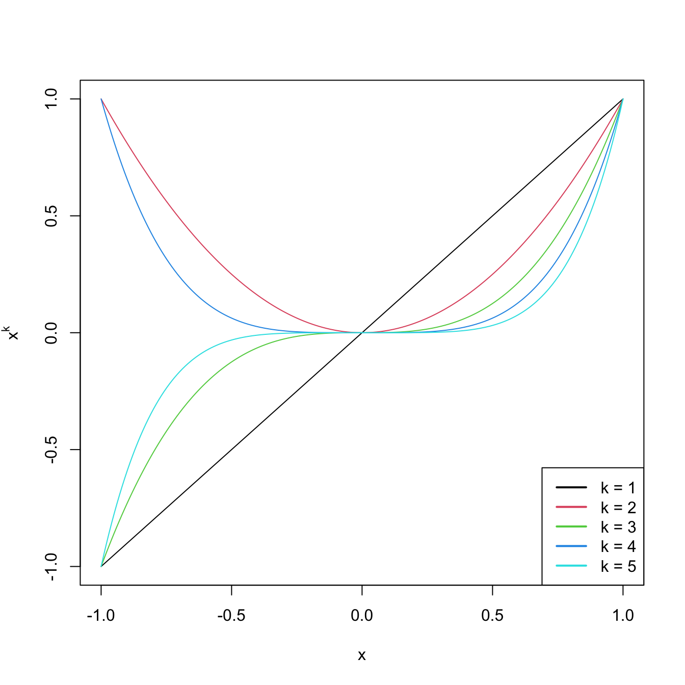

$Raw polynomials $x^k$ in $(-1,1),$ up to degree $k=5.$$

Figure 3.9: Raw polynomials $x^k$ in $(-1,1),$ up to degree $k=5.$

# Depiction of orthogonal polynomials
matplot(x, poly(x, degree = degree), type = "l", lty = 1,
        ylab = expression(p[k](x)))
legend("bottomright", legend = paste("k =", 1:degree), col = 1:degree, lwd = 2)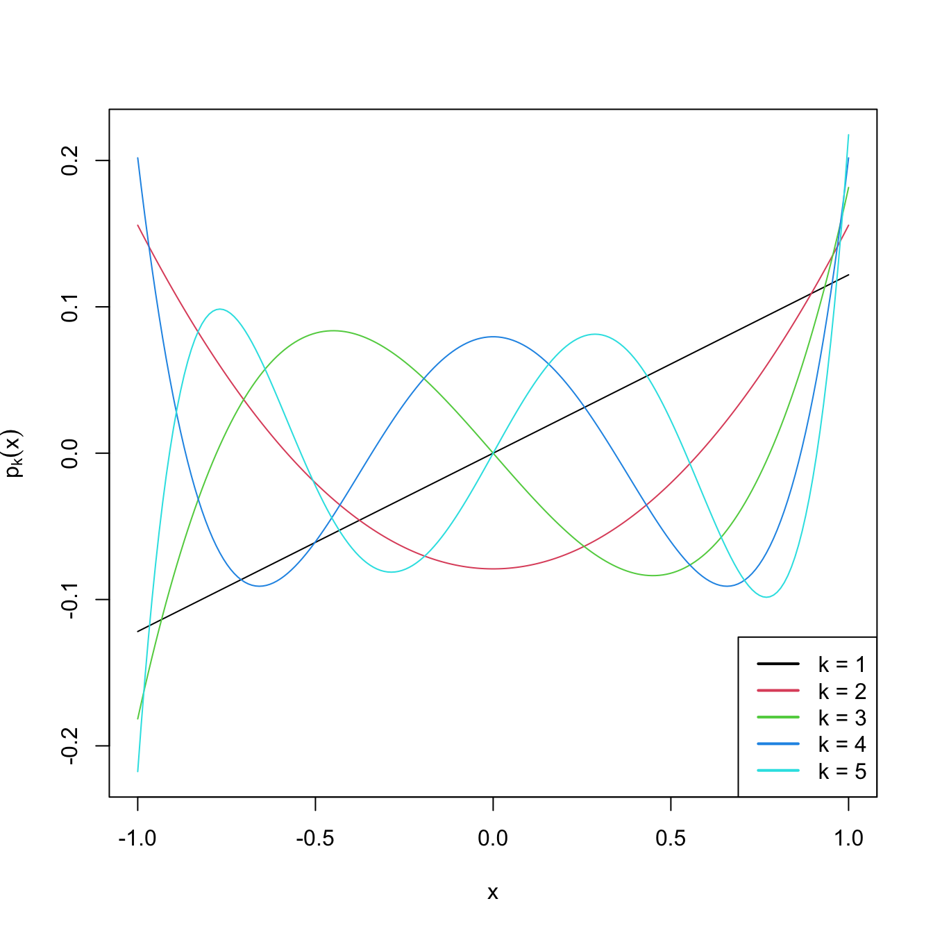

$Orthogonal polynomials $p_k(x)$ in $(-1,1),$ up to degree $k=5.$$

Figure 3.10: Orthogonal polynomials $p_k(x)$ in $(-1,1),$ up to degree $k=5.$

These matrices can now be used as inputs in the predictor side of lm. Let’s see this in an example.

# Data containing speed (mph) and stopping distance (ft) of cars from 1920
data(cars)
plot(cars, xlab = "Speed (mph)", ylab = "Stopping distance (ft)")

# Fit a linear model of dist ~ speed
mod1 <- lm(dist ~ speed, data = cars)
abline(coef = mod1$coefficients, col = 2)

# Quadratic
mod2 <- lm(dist ~ poly(speed, degree = 2), data = cars)
# The fit is not a line, we must look for an alternative approach
d <- seq(0, 25, length.out = 200)
lines(d, predict(mod2, new = data.frame(speed = d)), col = 3)

# Cubic
mod3 <- lm(dist ~ poly(speed, degree = 3), data = cars)
lines(d, predict(mod3, new = data.frame(speed = d)), col = 4)

# 10th order -- overfitting
mod10 <- lm(dist ~ poly(speed, degree = 10), data = cars)
lines(d, predict(mod10, new = data.frame(speed = d)), col = 5)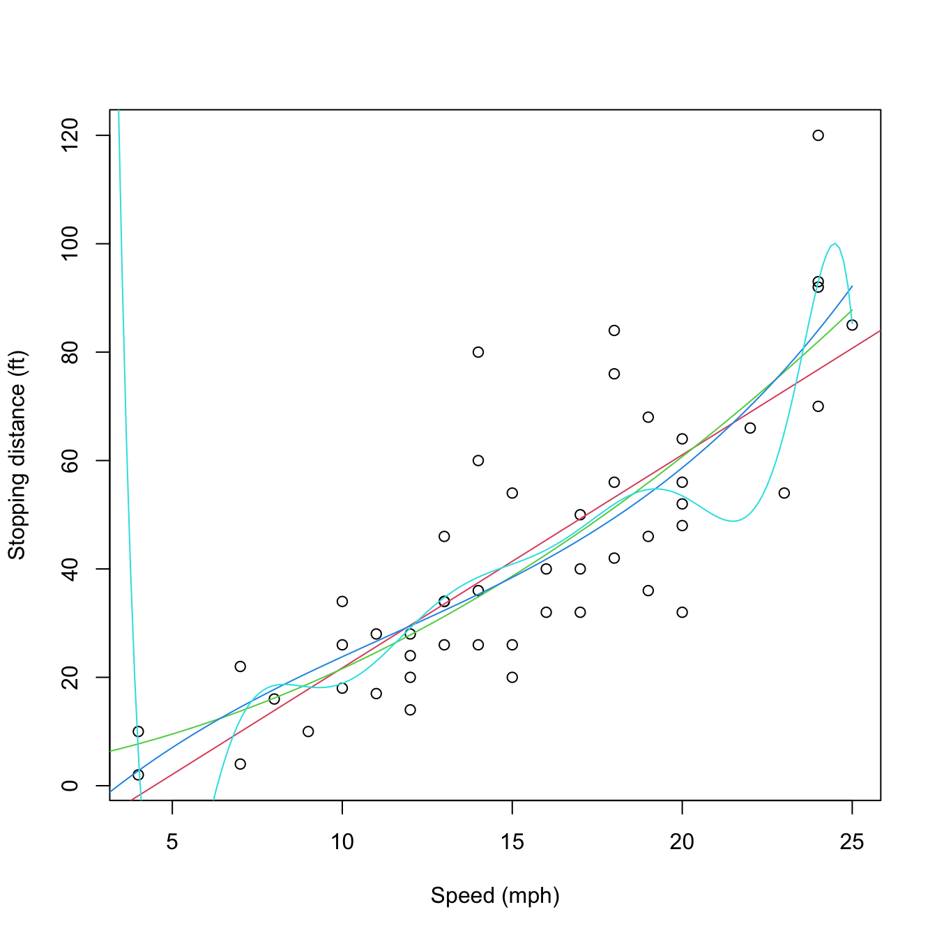

Figure 3.11: Raw and orthogonal polynomial fits of dist ~ speed in the cars dataset.


# BICs -- the linear model is better!
BIC(mod1, mod2, mod3, mod10)
##       df      BIC
## mod1   3 424.8929
## mod2   4 426.4202
## mod3   5 429.4451
## mod10 12 450.3523

# poly computes by default orthogonal polynomials. These are not
# X^1, X^2, ..., X^p but combinations of them such that the polynomials are
# orthogonal. 'Raw' polynomials are possible with raw = TRUE. They give the
# same fit, but the coefficient estimates are different.
mod2Raw <- lm(dist ~ poly(speed, degree = 2, raw = TRUE), data = cars)
plot(cars, xlab = "Speed (mph)", ylab = "Stopping distance (ft)")
lines(d, predict(mod2, new = data.frame(speed = d)), col = 1)
lines(d, predict(mod2Raw, new = data.frame(speed = d)), col = 2)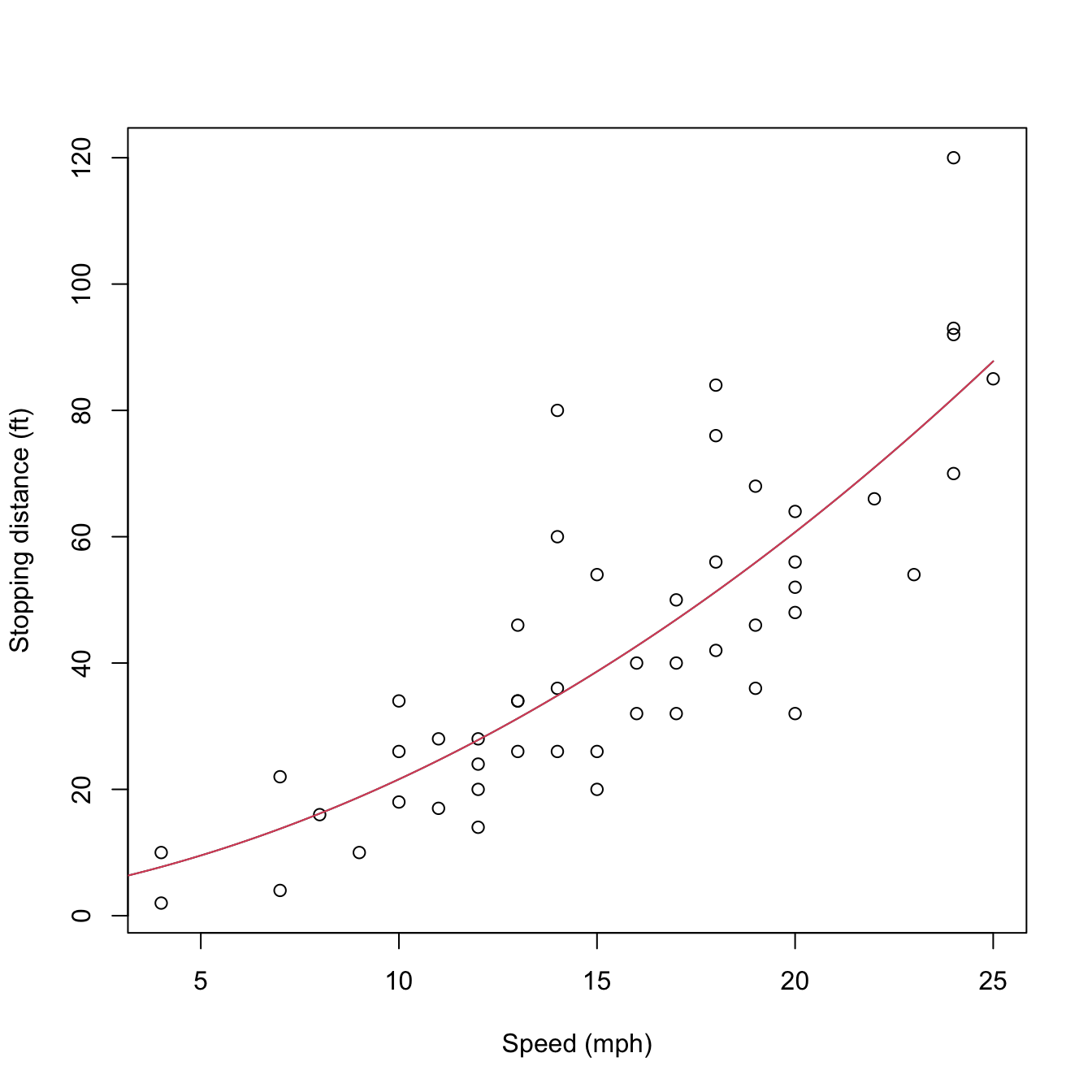

Figure 3.12: Raw and orthogonal polynomial fits of dist ~ speed in the cars dataset.

# However: different coefficient estimates, but same R^2. How is this possible?
summary(mod2)
## 
## Call:
## lm(formula = dist ~ poly(speed, degree = 2), data = cars)
## 
## Residuals:
##     Min      1Q  Median      3Q     Max 
## -28.720  -9.184  -3.188   4.628  45.152 
## 
## Coefficients:
##                          Estimate Std. Error t value Pr(>|t|)    
## (Intercept)                42.980      2.146  20.026  < 2e-16 ***
## poly(speed, degree = 2)1  145.552     15.176   9.591 1.21e-12 ***
## poly(speed, degree = 2)2   22.996     15.176   1.515    0.136    
## ---
## Signif. codes:  0 '***' 0.001 '**' 0.01 '*' 0.05 '.' 0.1 ' ' 1
## 
## Residual standard error: 15.18 on 47 degrees of freedom
## Multiple R-squared:  0.6673, Adjusted R-squared:  0.6532 
## F-statistic: 47.14 on 2 and 47 DF,  p-value: 5.852e-12
summary(mod2Raw)
## 
## Call:
## lm(formula = dist ~ poly(speed, degree = 2, raw = TRUE), data = cars)
## 
## Residuals:
##     Min      1Q  Median      3Q     Max 
## -28.720  -9.184  -3.188   4.628  45.152 
## 
## Coefficients:
##                                      Estimate Std. Error t value Pr(>|t|)
## (Intercept)                           2.47014   14.81716   0.167    0.868
## poly(speed, degree = 2, raw = TRUE)1  0.91329    2.03422   0.449    0.656
## poly(speed, degree = 2, raw = TRUE)2  0.09996    0.06597   1.515    0.136
## 
## Residual standard error: 15.18 on 47 degrees of freedom
## Multiple R-squared:  0.6673, Adjusted R-squared:  0.6532 
## F-statistic: 47.14 on 2 and 47 DF,  p-value: 5.852e-12

# Because the predictors in mod2Raw are highly related between them, and
# the ones in mod2 are uncorrelated between them!
car::scatterplotMatrix(mod2$model[, -1], col = 1, regLine = list(col = 2),
                       smooth = list(col.smooth = 4, col.spread = 4))
car::scatterplotMatrix(mod2Raw$model[, -1],col = 1, regLine = list(col = 2),
                       smooth = list(col.smooth = 4, col.spread = 4))
cor(mod2$model[, -1])
##   1 2
## 1 1 0
## 2 0 1
cor(mod2Raw$model[, -1])
##           1         2
## 1 1.0000000 0.9794765
## 2 0.9794765 1.0000000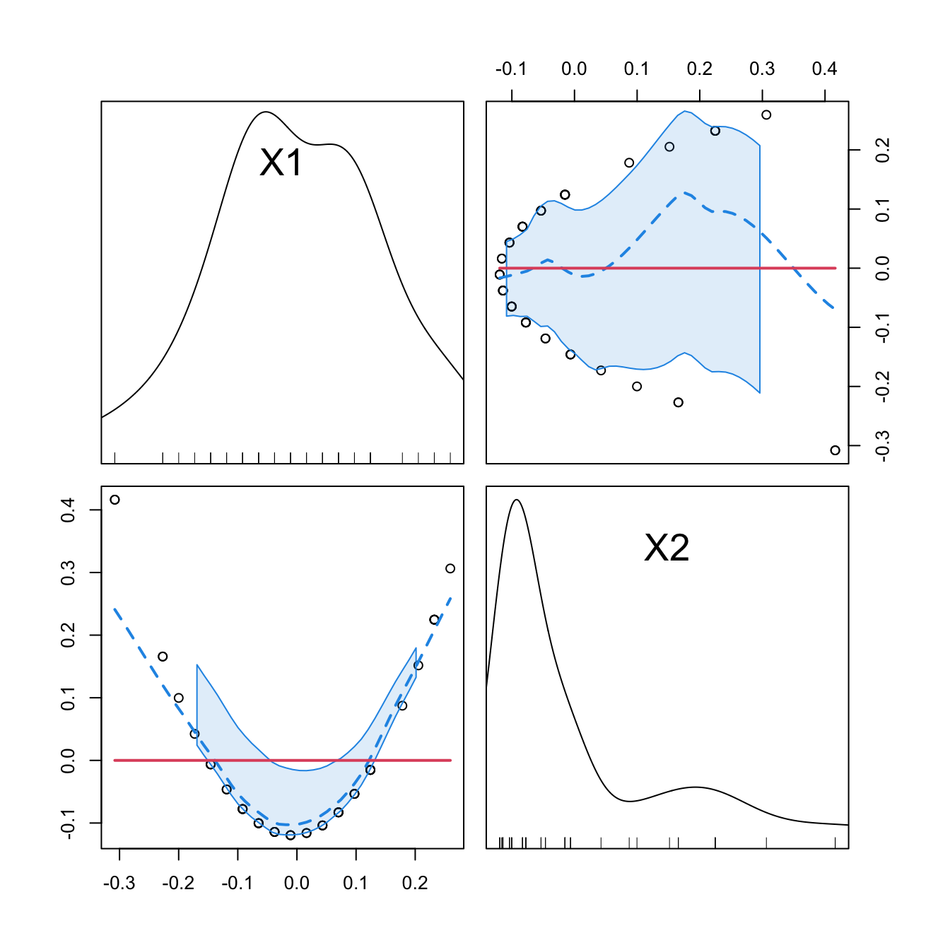

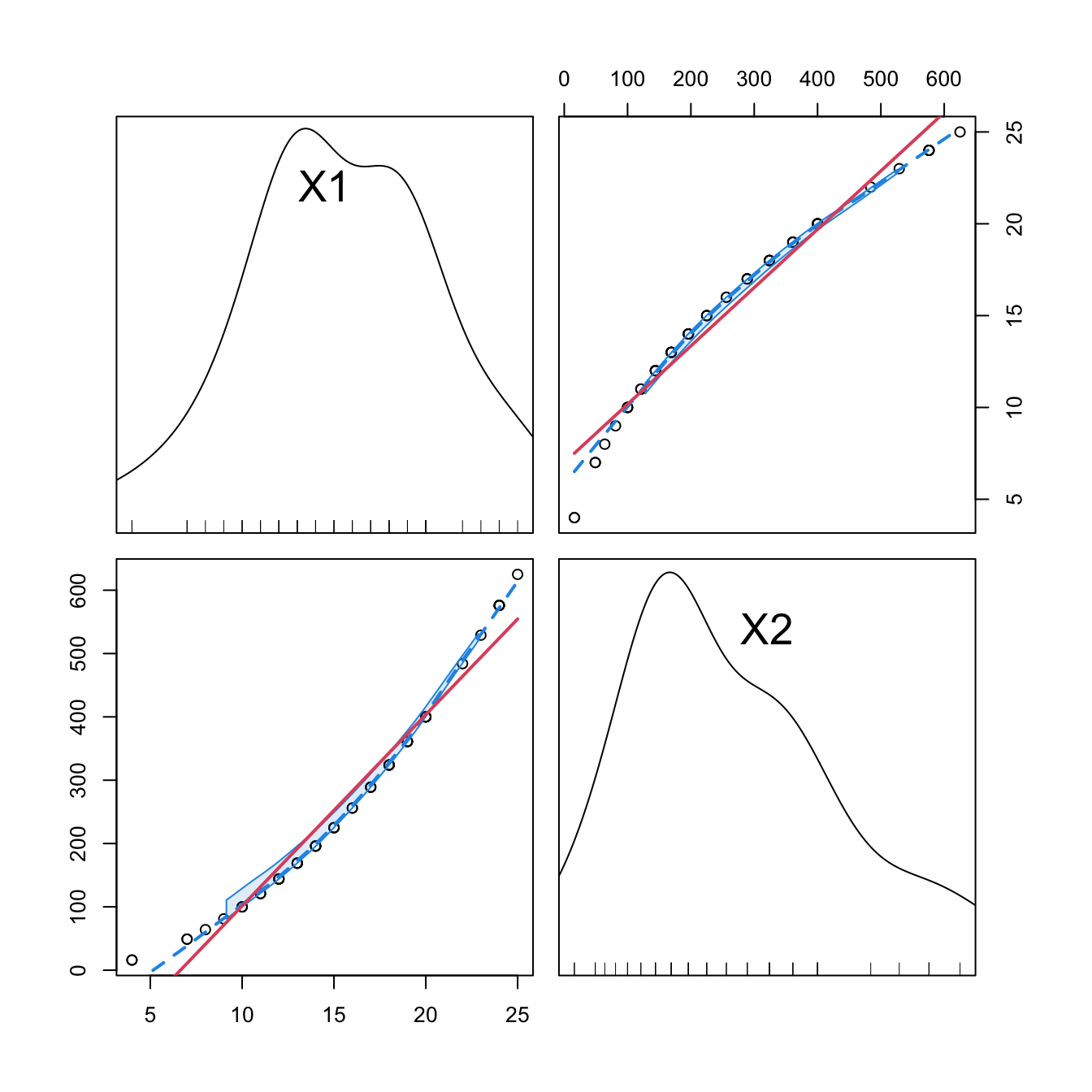
Figure 3.13: Correlations between the first and second order orthogonal polynomials associated to speed, and between speed and speed^2.

The use of orthogonal polynomials instead of raw polynomials is advised for high order polynomial fits, since they avoid the numerical instabilities arising from excessive linear dependencies between the raw polynomial predictors.

3.4.3 Interactions

When two or more predictors $X_1$ and $X_2$ are present, it may be of interest to explore the interaction between them by means of $X_1X_2.$ This is a new variable that positively (negatively) affects the response $Y$ when both $X_1$ and $X_2$ are positive or negative at the same time (at different times):

\[\begin{align*} Y=\beta_0+\beta_1X_1+\beta_2X_2+\beta_3X_1X_2+\varepsilon. \end{align*}\]

The coefficient $\beta_3$ in $Y=\beta_0+\beta_1X_1+\beta_2X_2+\beta_3X_1X_2+\varepsilon$ can be interpreted as the increment of the effect of the predictor $X_1$ on the mean of $Y,$ for a unit increment in $X_2$⁶⁷. Significance testing on these coefficients can be carried out as usual.

The way of adding these interactions in lm is through the operators : and *. The operator : only adds the term $X_1X_2,$ while * adds $X_1,$ $X_2,$ and $X_1X_2$ at the same time. Let’s see an example in the Boston dataset.

# Interaction between lstat and age
summary(lm(medv ~ lstat + lstat:age, data = Boston))
## 
## Call:
## lm(formula = medv ~ lstat + lstat:age, data = Boston)
## 
## Residuals:
##     Min      1Q  Median      3Q     Max 
## -15.815  -4.039  -1.335   2.086  27.491 
## 
## Coefficients:
##              Estimate Std. Error t value Pr(>|t|)    
## (Intercept) 36.041514   0.691334  52.133  < 2e-16 ***
## lstat       -1.388161   0.126911 -10.938  < 2e-16 ***
## lstat:age    0.004103   0.001133   3.621 0.000324 ***
## ---
## Signif. codes:  0 '***' 0.001 '**' 0.01 '*' 0.05 '.' 0.1 ' ' 1
## 
## Residual standard error: 6.142 on 503 degrees of freedom
## Multiple R-squared:  0.5557, Adjusted R-squared:  0.554 
## F-statistic: 314.6 on 2 and 503 DF,  p-value: < 2.2e-16
# For a unit increment in age, the effect of lstat in the response
# increases positively by 0.004103 units, shifting from -1.388161 to -1.384058

# Thus, when age increases makes lstat affect less negatively medv.
# Note that the same interpretation does NOT hold if we switch the roles
# of age and lstat because age is not present as a sole predictor!

# First order interaction
summary(lm(medv ~ lstat * age, data = Boston))
## 
## Call:
## lm(formula = medv ~ lstat * age, data = Boston)
## 
## Residuals:
##     Min      1Q  Median      3Q     Max 
## -15.806  -4.045  -1.333   2.085  27.552 
## 
## Coefficients:
##               Estimate Std. Error t value Pr(>|t|)    
## (Intercept) 36.0885359  1.4698355  24.553  < 2e-16 ***
## lstat       -1.3921168  0.1674555  -8.313 8.78e-16 ***
## age         -0.0007209  0.0198792  -0.036   0.9711    
## lstat:age    0.0041560  0.0018518   2.244   0.0252 *  
## ---
## Signif. codes:  0 '***' 0.001 '**' 0.01 '*' 0.05 '.' 0.1 ' ' 1
## 
## Residual standard error: 6.149 on 502 degrees of freedom
## Multiple R-squared:  0.5557, Adjusted R-squared:  0.5531 
## F-statistic: 209.3 on 3 and 502 DF,  p-value: < 2.2e-16

# Second order interaction
summary(lm(medv ~ lstat * age * indus, data = Boston))
## 
## Call:
## lm(formula = medv ~ lstat * age * indus, data = Boston)
## 
## Residuals:
##      Min       1Q   Median       3Q      Max 
## -15.1549  -3.6437  -0.8427   2.1991  24.8751 
## 
## Coefficients:
##                  Estimate Std. Error t value Pr(>|t|)    
## (Intercept)     46.103752   2.891173  15.946  < 2e-16 ***
## lstat           -2.641475   0.372223  -7.096 4.43e-12 ***
## age             -0.042300   0.041668  -1.015  0.31051    
## indus           -1.849829   0.380252  -4.865 1.54e-06 ***
## lstat:age        0.014249   0.004437   3.211  0.00141 ** 
## lstat:indus      0.177418   0.037647   4.713 3.18e-06 ***
## age:indus        0.014332   0.004386   3.268  0.00116 ** 
## lstat:age:indus -0.001621   0.000408  -3.973 8.14e-05 ***
## ---
## Signif. codes:  0 '***' 0.001 '**' 0.01 '*' 0.05 '.' 0.1 ' ' 1
## 
## Residual standard error: 5.929 on 498 degrees of freedom
## Multiple R-squared:  0.5901, Adjusted R-squared:  0.5844 
## F-statistic: 102.4 on 7 and 498 DF,  p-value: < 2.2e-16

A fast way of accounting interactions between predictors is to use the ^ operator in lm:

lm(y ~ (x1 + x2 + x3)^2) equals lm(y ~ x1 + x2 + x3 + x1:x2 + x1:x3 + x2:x3). Higher powers like lm(y ~ (x1 + x2 + x3)^3) include up to second-order interactions like x1:x2:x3.
It is possible to regress on all the predictors and the first order interactions using lm(y ~ .^2).
Further flexibility in lm is possible, e.g., removing a particular interaction with lm(y ~ .^2 - x1:x2) or forcing the intercept to be zero with lm(y ~ 0 + .^2).

Stepwise regression can also be performed with interaction terms. MASS::stepAIC supports interaction terms, but their inclusion must be asked for in the scope argument. By default, scope considers the largest model in which to perform stepwise regression as the formula of the model in object, the first argument. In order to set the largest model to search for the best subset of predictors as the one that contains first-order interactions, we proceed as follows:

# Include first-order interactions in the search for the best model in
# terms of BIC, not just single predictors
modIntBIC <- MASS::stepAIC(object = lm(medv ~ ., data = Boston),
                           scope = medv ~ .^2, k = log(nobs(modBIC)), trace = 0)
summary(modIntBIC)
## 
## Call:
## lm(formula = medv ~ crim + indus + chas + nox + rm + age + dis + 
##     rad + tax + ptratio + black + lstat + rm:lstat + rad:lstat + 
##     rm:rad + dis:rad + black:lstat + dis:ptratio + crim:chas + 
##     chas:nox + chas:rm + chas:ptratio + rm:ptratio + age:black + 
##     indus:dis + indus:lstat + crim:rm + crim:lstat, data = Boston)
## 
## Residuals:
##     Min      1Q  Median      3Q     Max 
## -8.5845 -1.6797 -0.3157  1.5433 19.4311 
## 
## Coefficients:
##                Estimate Std. Error t value Pr(>|t|)    
## (Intercept)  -9.673e+01  1.350e+01  -7.167 2.93e-12 ***
## crim         -1.454e+00  3.147e-01  -4.620 4.95e-06 ***
## indus         7.647e-01  1.237e-01   6.182 1.36e-09 ***
## chas          6.341e+01  1.115e+01   5.687 2.26e-08 ***
## nox          -1.691e+01  3.020e+00  -5.598 3.67e-08 ***
## rm            1.946e+01  1.730e+00  11.250  < 2e-16 ***
## age           2.233e-01  5.898e-02   3.786 0.000172 ***
## dis          -2.462e+00  6.776e-01  -3.634 0.000309 ***
## rad           3.461e+00  3.109e-01  11.132  < 2e-16 ***
## tax          -1.401e-02  2.536e-03  -5.522 5.52e-08 ***
## ptratio       1.207e+00  7.085e-01   1.704 0.089111 .  
## black         7.946e-02  1.262e-02   6.298 6.87e-10 ***
## lstat         2.939e+00  2.707e-01  10.857  < 2e-16 ***
## rm:lstat     -3.793e-01  3.592e-02 -10.559  < 2e-16 ***
## rad:lstat    -4.804e-02  4.465e-03 -10.760  < 2e-16 ***
## rm:rad       -3.490e-01  4.370e-02  -7.986 1.05e-14 ***
## dis:rad      -9.236e-02  2.603e-02  -3.548 0.000427 ***
## black:lstat  -8.337e-04  3.355e-04  -2.485 0.013292 *  
## dis:ptratio   1.371e-01  3.719e-02   3.686 0.000254 ***
## crim:chas     2.544e+00  3.813e-01   6.672 7.01e-11 ***
## chas:nox     -3.706e+01  6.202e+00  -5.976 4.48e-09 ***
## chas:rm      -3.774e+00  7.402e-01  -5.099 4.94e-07 ***
## chas:ptratio -1.185e+00  3.701e-01  -3.203 0.001451 ** 
## rm:ptratio   -3.792e-01  1.067e-01  -3.555 0.000415 ***
## age:black    -7.107e-04  1.552e-04  -4.578 5.99e-06 ***
## indus:dis    -1.316e-01  2.533e-02  -5.197 3.00e-07 ***
## indus:lstat  -2.580e-02  5.204e-03  -4.959 9.88e-07 ***
## crim:rm       1.605e-01  4.001e-02   4.011 7.00e-05 ***
## crim:lstat    1.511e-02  4.954e-03   3.051 0.002408 ** 
## ---
## Signif. codes:  0 '***' 0.001 '**' 0.01 '*' 0.05 '.' 0.1 ' ' 1
## 
## Residual standard error: 3.045 on 477 degrees of freedom
## Multiple R-squared:  0.8964, Adjusted R-squared:  0.8904 
## F-statistic: 147.5 on 28 and 477 DF,  p-value: < 2.2e-16

# There is no improvement by removing terms in modIntBIC
MASS::dropterm(modIntBIC, k = log(nobs(modIntBIC)), sorted = TRUE)
## Single term deletions
## 
## Model:
## medv ~ crim + indus + chas + nox + rm + age + dis + rad + tax + 
##     ptratio + black + lstat + rm:lstat + rad:lstat + rm:rad + 
##     dis:rad + black:lstat + dis:ptratio + crim:chas + chas:nox + 
##     chas:rm + chas:ptratio + rm:ptratio + age:black + indus:dis + 
##     indus:lstat + crim:rm + crim:lstat
##              Df Sum of Sq    RSS    AIC
## <none>                    4423.7 1277.7
## black:lstat   1     57.28 4481.0 1278.0
## crim:lstat    1     86.33 4510.1 1281.2
## chas:ptratio  1     95.15 4518.9 1282.2
## dis:rad       1    116.73 4540.5 1284.6
## rm:ptratio    1    117.23 4541.0 1284.7
## dis:ptratio   1    126.00 4549.7 1285.7
## crim:rm       1    149.24 4573.0 1288.2
## age:black     1    194.40 4618.1 1293.2
## indus:lstat   1    228.05 4651.8 1296.9
## chas:rm       1    241.11 4664.8 1298.3
## indus:dis     1    250.51 4674.2 1299.3
## tax           1    282.77 4706.5 1302.8
## chas:nox      1    331.19 4754.9 1308.0
## crim:chas     1    412.86 4836.6 1316.6
## rm:rad        1    591.45 5015.2 1335.0
## rm:lstat      1   1033.93 5457.7 1377.7
## rad:lstat     1   1073.80 5497.5 1381.4

# Neither by including other terms interactions
MASS::addterm(modIntBIC, scope = lm(medv ~ .^2, data = Boston),
              k = log(nobs(modIntBIC)), sorted = TRUE)
## Single term additions
## 
## Model:
## medv ~ crim + indus + chas + nox + rm + age + dis + rad + tax + 
##     ptratio + black + lstat + rm:lstat + rad:lstat + rm:rad + 
##     dis:rad + black:lstat + dis:ptratio + crim:chas + chas:nox + 
##     chas:rm + chas:ptratio + rm:ptratio + age:black + indus:dis + 
##     indus:lstat + crim:rm + crim:lstat
##               Df Sum of Sq    RSS    AIC
## <none>                     4423.7 1277.7
## nox:age        1    52.205 4371.5 1277.9
## chas:lstat     1    50.231 4373.5 1278.1
## crim:nox       1    50.002 4373.7 1278.2
## indus:tax      1    46.182 4377.6 1278.6
## nox:rad        1    42.822 4380.9 1279.0
## tax:ptratio    1    37.105 4386.6 1279.6
## age:lstat      1    29.825 4393.9 1280.5
## rm:tax         1    27.221 4396.5 1280.8
## nox:rm         1    25.099 4398.6 1281.0
## nox:ptratio    1    17.994 4405.7 1281.8
## rm:age         1    16.956 4406.8 1282.0
## crim:black     1    15.566 4408.2 1282.1
## dis:tax        1    13.336 4410.4 1282.4
## dis:lstat      1    10.944 4412.8 1282.7
## rm:black       1     9.909 4413.8 1282.8
## rm:dis         1     9.312 4414.4 1282.8
## crim:indus     1     8.458 4415.3 1282.9
## tax:lstat      1     7.891 4415.8 1283.0
## ptratio:black  1     7.769 4416.0 1283.0
## rad:black      1     7.327 4416.4 1283.1
## age:ptratio    1     6.857 4416.9 1283.1
## age:tax        1     5.785 4417.9 1283.2
## nox:dis        1     5.727 4418.0 1283.2
## age:dis        1     5.618 4418.1 1283.3
## nox:tax        1     5.579 4418.2 1283.3
## crim:dis       1     5.376 4418.4 1283.3
## tax:black      1     4.867 4418.9 1283.3
## indus:age      1     4.554 4419.2 1283.4
## indus:rm       1     4.089 4419.6 1283.4
## indus:ptratio  1     4.082 4419.6 1283.4
## zn             1     3.919 4419.8 1283.5
## chas:tax       1     3.918 4419.8 1283.5
## rad:tax        1     3.155 4420.6 1283.5
## age:rad        1     3.085 4420.6 1283.5
## nox:black      1     2.939 4420.8 1283.6
## ptratio:lstat  1     2.469 4421.3 1283.6
## indus:chas     1     2.359 4421.4 1283.6
## chas:black     1     1.940 4421.8 1283.7
## indus:nox      1     1.440 4422.3 1283.7
## indus:black    1     1.177 4422.6 1283.8
## chas:rad       1     0.757 4423.0 1283.8
## chas:age       1     0.757 4423.0 1283.8
## crim:rad       1     0.678 4423.1 1283.8
## nox:lstat      1     0.607 4423.1 1283.8
## rad:ptratio    1     0.567 4423.2 1283.8
## crim:age       1     0.348 4423.4 1283.9
## indus:rad      1     0.219 4423.5 1283.9
## dis:black      1     0.077 4423.7 1283.9
## crim:ptratio   1     0.019 4423.7 1283.9
## crim:tax       1     0.004 4423.7 1283.9
## chas:dis       1     0.004 4423.7 1283.9

Interactions are also possible with categorical variables. For example, for one predictor $X$ and one dummy variable $D$ encoding a factor with two levels, we have seven possible linear models stemming from how we want to combine $X$ and $D.$ Outlining these models helps understanding the possible range of effects of adding a dummy variable:

Predictor and no dummy variable. The usual simple linear model:

\[\begin{align*} Y=\beta_0+\beta_1X+\varepsilon \end{align*}\]

Predictor and dummy variable. $D$ affects the intercept of the linear model, which is different for each group:

\[\begin{align*} Y=\beta_0+\beta_1X+\beta_2D+\varepsilon=\begin{cases}\beta_0+\beta_1X+\varepsilon,&\text{if }D=0,\\(\beta_0+\beta_2)+\beta_1X+\varepsilon,&\text{if }D=1.\end{cases} \end{align*}\]

Predictor and dummy variable, with interaction. $D$ affects the intercept and the slope of the linear model, and both are different for each group:

\[\begin{align*} Y&=\beta_0+\beta_1X+\beta_2D+\beta_3(X\cdot D)+\varepsilon\\ &=\begin{cases}\beta_0+\beta_1X+\varepsilon,&\text{if }D=0,\\(\beta_0+\beta_2)+(\beta_1+\beta_3)X+\varepsilon,&\text{if }D=1.\end{cases} \end{align*}\]

Predictor and interaction with dummy variable. $D$ affects only the slope of the linear model, which is different for each group:

\[\begin{align*} Y=\beta_0+\beta_1X+\beta_2(X\cdot D)+\varepsilon=\begin{cases}\beta_0+\beta_1X+\varepsilon,&\text{if }D=0,\\\beta_0+(\beta_1+\beta_2)X+\varepsilon,&\text{if }D=1.\end{cases} \end{align*}\]

Dummy variable and no predictor. $D$ controls the intercept of a constant fit, depending on each group:

\[\begin{align*} Y=\beta_0+\beta_1 D+\varepsilon=\begin{cases}\beta_0+\varepsilon,&\text{if }D=0,\\(\beta_0+\beta_1)+\varepsilon,&\text{if }D=1.\end{cases} \end{align*}\]

Dummy variable and interaction with predictor. $D$ adds the predictor $X$ for one group and affects the intercept, which is different for each group:

\[\begin{align*} Y=\beta_0+\beta_1D+\beta_2(X\cdot D)+\varepsilon=\begin{cases}\beta_0+\varepsilon,&\text{if }D=0,\\(\beta_0+\beta_1)+\beta_2X+\varepsilon,&\text{if }D=1.\end{cases} \end{align*}\]

Interaction of dummy and predictor. $D$ adds the predictor $X$ for one group and the intercept is common:

\[\begin{align*} Y=\beta_0+\beta_1(X\cdot D)+\varepsilon=\begin{cases}\beta_0+\varepsilon,&\text{if }D=0,\\\beta_0+\beta_1X+\varepsilon,&\text{if }D=1.\end{cases} \end{align*}\]

Let’s see the visualization of these seven models with $Y=$ medv, $X=$ lstat, and $D=$ chas for the Boston dataset. In the following, the green color stands for data points and linear fits associated to $D=0,$ whereas blue stands for $D=1.$

# Group settings
col <- Boston$chas + 3
cex <- 0.5 + 0.25 * Boston$chas

# 1. No dummy variable
(mod1 <- lm(medv ~ lstat, data = Boston))
## 
## Call:
## lm(formula = medv ~ lstat, data = Boston)
## 
## Coefficients:
## (Intercept)        lstat  
##       34.55        -0.95
plot(medv ~ lstat, data = Boston, col = col, pch = 16, cex = cex, main = "1")
abline(coef = mod1$coefficients, lwd = 2)


# 2. Dummy variable
(mod2 <- lm(medv ~ lstat + chas, data = Boston))
## 
## Call:
## lm(formula = medv ~ lstat + chas, data = Boston)
## 
## Coefficients:
## (Intercept)        lstat         chas  
##     34.0941      -0.9406       4.9200
plot(medv ~ lstat, data = Boston, col = col, pch = 16, cex = cex, main = "2")
abline(a = mod2$coefficients[1], b = mod2$coefficients[2], col = 3, lwd = 2)
abline(a = mod2$coefficients[1] + mod2$coefficients[3],
       b = mod2$coefficients[2], col = 4, lwd = 2)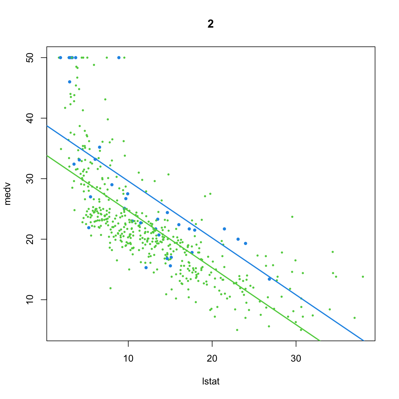


# 3. Dummy variable, with interaction
(mod3 <- lm(medv ~ lstat * chas, data = Boston))
## 
## Call:
## lm(formula = medv ~ lstat * chas, data = Boston)
## 
## Coefficients:
## (Intercept)        lstat         chas   lstat:chas  
##     33.7672      -0.9150       9.8251      -0.4329
plot(medv ~ lstat, data = Boston, col = col, pch = 16, cex = cex, main = "3")
abline(a = mod3$coefficients[1], b = mod3$coefficients[2], col = 3, lwd = 2)
abline(a = mod3$coefficients[1] + mod3$coefficients[3],
       b = mod3$coefficients[2] + mod3$coefficients[4], col = 4, lwd = 2)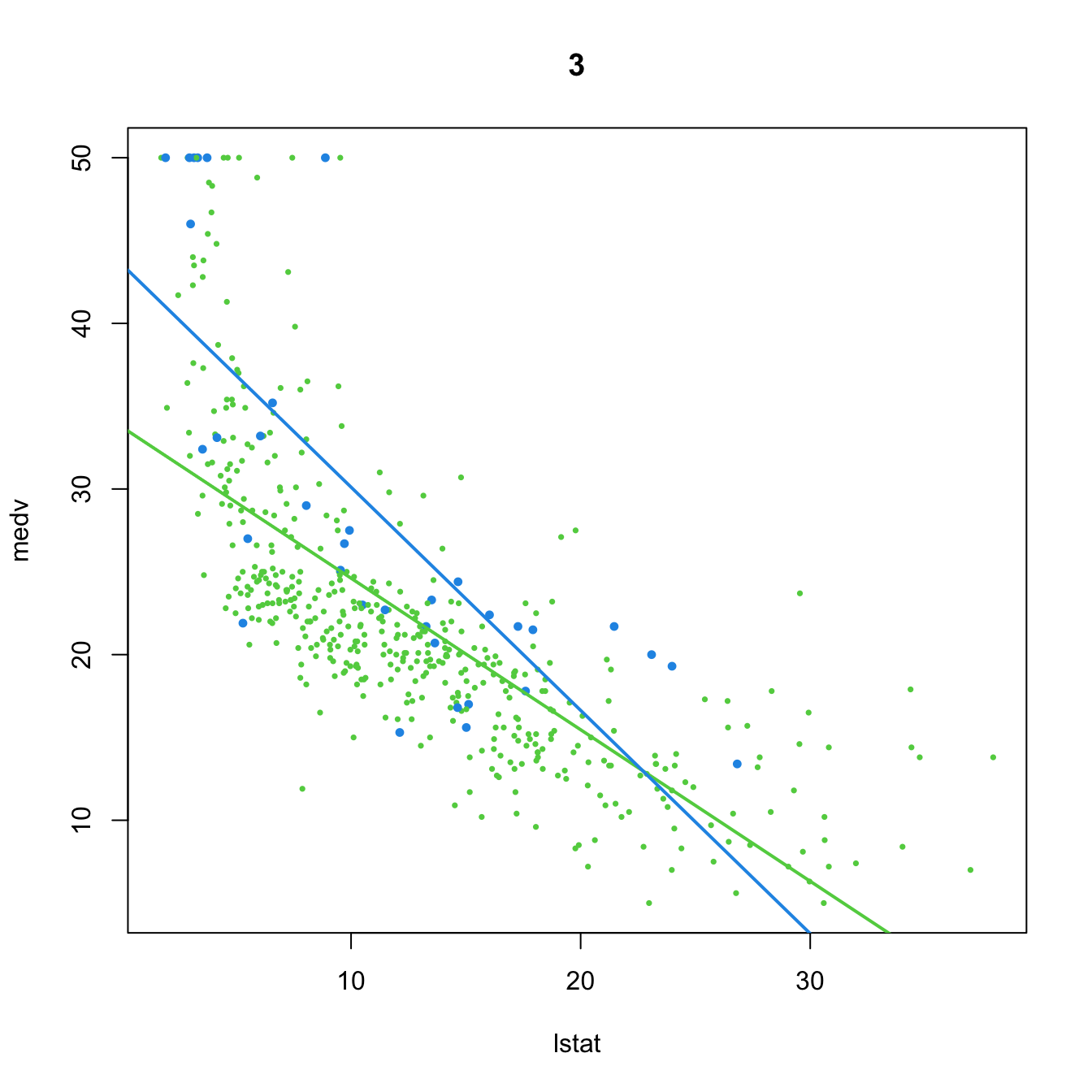


# 4. Dummy variable only present in interaction
(mod4 <- lm(medv ~ lstat + lstat:chas, data = Boston))
## 
## Call:
## lm(formula = medv ~ lstat + lstat:chas, data = Boston)
## 
## Coefficients:
## (Intercept)        lstat   lstat:chas  
##     34.4893      -0.9580       0.2128
plot(medv ~ lstat, data = Boston, col = col, pch = 16, cex = cex, main = "4")
abline(a = mod4$coefficients[1], b = mod4$coefficients[2], col = 3, lwd = 2)
abline(a = mod4$coefficients[1],
       b = mod4$coefficients[2] + mod4$coefficients[3], col = 4, lwd = 2)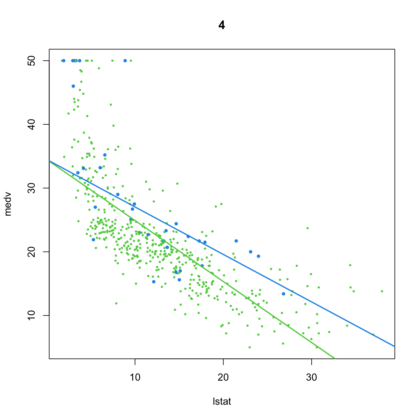


# 5. Dummy variable and no predictor
(mod5 <- lm(medv ~ chas, data = Boston))
## 
## Call:
## lm(formula = medv ~ chas, data = Boston)
## 
## Coefficients:
## (Intercept)         chas  
##      22.094        6.346
plot(medv ~ lstat, data = Boston, col = col, pch = 16, cex = cex, main = "5")
abline(a = mod5$coefficients[1], b = 0, col = 3, lwd = 2)
abline(a = mod5$coefficients[1] + mod5$coefficients[2], b = 0, col = 4, lwd = 2)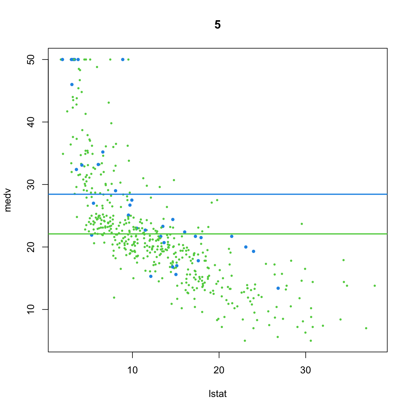


# 6. Dummy variable. Interaction in the intercept and slope
(mod6 <- lm(medv ~ chas + lstat:chas, data = Boston))
## 
## Call:
## lm(formula = medv ~ chas + lstat:chas, data = Boston)
## 
## Coefficients:
## (Intercept)         chas   chas:lstat  
##      22.094       21.498       -1.348
plot(medv ~ lstat, data = Boston, col = col, pch = 16, cex = cex, main = "6")
abline(a = mod6$coefficients[1], b = 0, col = 3, lwd = 2)
abline(a = mod6$coefficients[1] + mod6$coefficients[2],
       b = mod6$coefficients[3], col = 4, lwd = 2)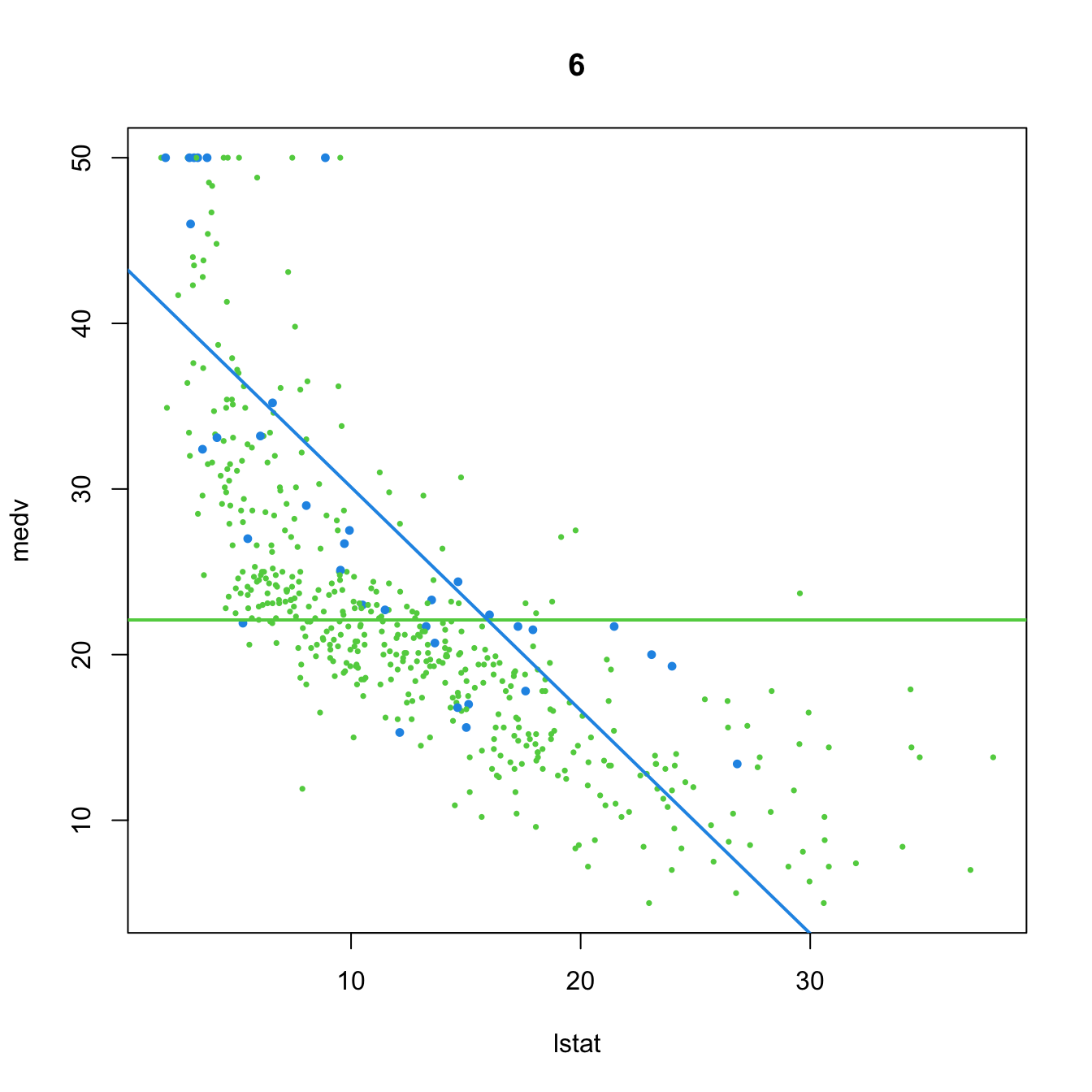


# 7. Dummy variable. Interaction in the slope
(mod7 <- lm(medv ~ lstat:chas, data = Boston))
## 
## Call:
## lm(formula = medv ~ lstat:chas, data = Boston)
## 
## Coefficients:
## (Intercept)   lstat:chas  
##    22.49484      0.04882
plot(medv ~ lstat, data = Boston, col = col, pch = 16, cex = cex, main = "7")
abline(a = mod7$coefficients[1], b = 0, col = 3, lwd = 2)
abline(a = mod7$coefficients[1], b = mod7$coefficients[2], col = 4, lwd = 2)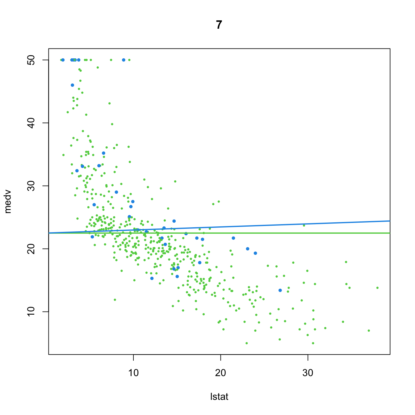

From the above illustration, it is clear that the effect of adding a dummy variable is to simultaneously fit two linear models (with varying flexibility) to the two groups of data encoded by the dummy variable, and merge this simultaneous fit within a single linear model. We can check this in more detail using the subset option of lm:

# Model using a dummy variable in the full dataset
lm(medv ~ lstat + chas + lstat:chas, data = Boston)
## 
## Call:
## lm(formula = medv ~ lstat + chas + lstat:chas, data = Boston)
## 
## Coefficients:
## (Intercept)        lstat         chas   lstat:chas  
##     33.7672      -0.9150       9.8251      -0.4329

# Individual model for the group with chas == 0
lm(medv ~ lstat, data = Boston, subset = chas == 0)
## 
## Call:
## lm(formula = medv ~ lstat, data = Boston, subset = chas == 0)
## 
## Coefficients:
## (Intercept)        lstat  
##      33.767       -0.915
# Notice that the intercept and lstat coefficient are the same as before

# Individual model for the group with chas == 1
lm(medv ~ lstat, data = Boston, subset = chas == 1)
## 
## Call:
## lm(formula = medv ~ lstat, data = Boston, subset = chas == 1)
## 
## Coefficients:
## (Intercept)        lstat  
##      43.592       -1.348
# Notice that the intercept and lstat coefficient equal the ones from the
# joint model, plus the specific terms associated to chas

This discussion can be extended to factors with several levels with more associated dummy variables. The next code chunk shows how three group-specific linear regressions are modeled together by means of two dummy variables in the iris dataset.

# Does not take into account the groups in the data
modIris <- lm(Sepal.Width ~ Petal.Width, data = iris)
modIris$coefficients
## (Intercept) Petal.Width 
##   3.3084256  -0.2093598

# Adding interactions with the groups
modIrisSpecies <- lm(Sepal.Width ~ Petal.Width * Species, data = iris)
modIrisSpecies$coefficients
##                   (Intercept)                   Petal.Width             Speciesversicolor              Speciesvirginica 
##                     3.2220507                     0.8371922                    -1.8491878                    -1.5272777 
## Petal.Width:Speciesversicolor  Petal.Width:Speciesvirginica 
##                     0.2164556                    -0.2057870

# Joint regression line shows negative correlation, but each group
# regression line shows a positive correlation
plot(Sepal.Width ~ Petal.Width, data = iris, col = as.integer(Species) + 1,
     pch = 16)
abline(a = modIris$coefficients[1], b = modIris$coefficients[2], lwd = 2)
abline(a = modIrisSpecies$coefficients[1], b = modIrisSpecies$coefficients[2],
       col = 2, lwd = 2)
abline(a = modIrisSpecies$coefficients[1] + modIrisSpecies$coefficients[3],
       b = modIrisSpecies$coefficients[2] + modIrisSpecies$coefficients[5],
       col = 3, lwd = 2)
abline(a = modIrisSpecies$coefficients[1] + modIrisSpecies$coefficients[4],
       b = modIrisSpecies$coefficients[2] + modIrisSpecies$coefficients[6],
       col = 4, lwd = 2)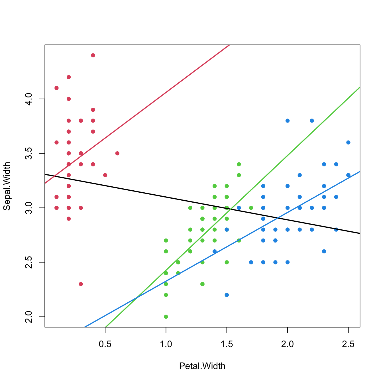

The three linear fits of Sepal.Width ~ Petal.Width * Species for each of the three levels in the Species factor (setosa in red, versicolor in green, and virginica in blue) in the iris dataset. The black line represents the linear fit for Sepal.Width ~ Petal.Width, that is, the linear fit without accounting for the levels in Species. Recall how Sepal.Widthis positively correlated with Petal.Width within each group, but is negatively correlated in the aggregated data.

Figure 3.14: The three linear fits of Sepal.Width ~ Petal.Width * Species for each of the three levels in the Species factor (setosa in red, versicolor in green, and virginica in blue) in the iris dataset. The black line represents the linear fit for Sepal.Width ~ Petal.Width, that is, the linear fit without accounting for the levels in Species. Recall how Sepal.Widthis positively correlated with Petal.Width within each group, but is negatively correlated in the aggregated data.

The last scatterplot is an illustration of the Simpson’s paradox. The simplest case of the paradox arises in simple linear regression, when there are two or more well-defined groups in the data such that:

Within each group, there is a clear and common correlation pattern between the response and the predictor.
When the groups are aggregated, the response and the predictor exhibit an opposite correlation pattern.

If groups are present in the data, always explore the intra-group correlations!

3.4.4 Case study application

The model employed in Harrison and Rubinfeld (1978) is different from the modBIC model. In the paper, several nonlinear transformations of the predictors and the response are done to improve the linear fit. Also, different units are used for medv, black, lstat, and nox. The authors considered these variables:

Response: log(1000 * medv).
Linear predictors: age, black / 1000 (this variable corresponds to their $(B-0.63)^2$), tax, ptratio, crim, zn, indus, and chas.
Nonlinear predictors: rm^2, log(dis), log(rad), log(lstat / 100), and (10 * nox)^2.

Do the following:

Check if the model with such predictors corresponds to the one in the first column, Table VII, page 100 of Harrison and Rubinfeld (1978) (open-access paper available here). To do so, save this model as modelHarrison and summarize it.
Make a stepAIC selection of the variables in modelHarrison (use BIC) and save it as modelHarrisonSel. Summarize the fit.
Which model has a larger $R^2$? And $R^2_\text{Adj}$? Which is simpler and has more significant coefficients?

References

Harrison, D., and D. L. Rubinfeld. 1978. “Hedonic Housing Prices and the Demand for Clean Air.” Journal of Environmental Economics and Management 5 (1): 81–102. https://doi.org/10.1016/0095-0696(78)90006-2.

In particular, Taylor’s theorem allows to approximate a sufficiently regular function $m$ by a polynomial, which is identifiable with a multiple linear model as seen in Section 3.4.2. This idea, applied locally, is elaborated in Section 6.2.2.↩︎
The consideration of more than one predictor is conceptually straightforward, yet notationally more cumbersome.↩︎
Precisely, the type of orthogonal polynomials considered are a data-driven shifting and rescaling of the Legendre polynomials in $(-1,1).$ The Legendre polynomials $p_j$ and $p_\ell$ in $(-1,1)$ satisfy that $\int_{-1}^1 p_j(x)p_\ell(x)\,\mathrm{d}x=\frac{2}{2j+1}\delta_{j\ell},$ where $\delta_{j\ell}$ is the Kronecker’s delta. The first five Legendre polynomials in $(-1,1)$ are, respectively: $p_1(x)=x,$ $p_2(x)=\frac{1}{2}(3x^2-1),$ $p_3(x)=\frac{1}{2}(5x^3-3x),$ $p_4(x)=\frac{1}{8}(35x^4-30x^2+3),$ and $p_5(x)=\frac{1}{8}(63x^5-70x^3+15x).$ Also, $p_0(x)=1.$ The recursive formula $p_{k+1}(x)=(k+1)^{-1}\big[(2k+1)xp_k(x)-kp_{k-1}(x)\big]$ allows to obtain the $(k+1)$-th order Legendre polynomial from the previous two ones. Notice that from $k\geq 3,$ $p_k(x)$ involves more monomials than just $x^k,$ precisely all the monomials with a lower order and with the same parity. This may complicate the interpretation of a coefficient related to $p_k(X)$ for $k\geq3,$ as it is not directly associated to a $k$-th order effect of $X.$↩︎
This is due to how the second matrix of (3.5) is computed: by means of a $QR$ decomposition associated to the first matrix. The decomposition yields a data matrix formed by polynomials that are not exactly the Legendre polynomials but a data-driven shifting and rescaling of them.↩︎
Of course, the roles of $X_1$ and $X_2$ can be interchanged in this interpretation.↩︎