4.4 Big data considerations
The computation of the least squares estimator
\[\begin{align} \hat{\boldsymbol{\beta}}=(\mathbf{X}'\mathbf{X})^{-1}\mathbf{X}'\mathbf{Y}\tag{4.24} \end{align}\]
involves inverting the \((p+1)\times(p+1)\) matrix \(\mathbf{X}'\mathbf{X},\) where \(\mathbf{X}\) is an \(n\times(p+1)\) matrix. The vector to be obtained, \(\hat{\boldsymbol{\beta}},\) is of size \(p+1.\) However, computing it directly from (4.24) requires allocating \(\mathcal{O}(np + p^2)\) elements in memory. When \(n\) is very large, this can be prohibitive. In addition, for convenience of the statistical analysis, R’s lm returns several objects of the same size as \(\mathbf{X}\) and \(\mathbf{Y},\) thus notably increasing the memory usage. For these reasons, alternative approaches for computing \(\hat{\boldsymbol{\beta}}\) with big data are required.
An approach for computing (4.24) in a memory-friendly way is to split the computation of \((\mathbf{X}'\mathbf{X})^{-1}\) and \(\mathbf{X}'\mathbf{Y}\) by blocks that are storable in memory. A possibility is to update sequentially the estimation of the vector of coefficients. This can be done with the following expression, which relates \(\hat{\boldsymbol{\beta}}\) with \(\hat{\boldsymbol{\beta}}_{-i},\) the vector of estimated coefficients without the \(i\)-th datum:
\[\begin{align} \hat{\boldsymbol{\beta}}=\hat{\boldsymbol{\beta}}_{-i}+(\mathbf{X}'\mathbf{X})^{-1}\mathbf{x}_{i}\left(Y_{i}-\mathbf{x}_{i}'\hat{\boldsymbol{\beta}}_{-i}\right).\tag{4.25} \end{align}\]
In (4.25) above, \(\mathbf{x}_{i}'\) is the \(i\)-th row of the design matrix \(\mathbf{X}.\) The expression follows from the Sherman–Morrison formula for an invertible matrix \(\mathbf{A}\) and a vector \(\mathbf{b},\)
\[\begin{align*} (\mathbf{A}+\mathbf{b}\mathbf{b}')^{-1}=\mathbf{A}^{-1}-\frac{\mathbf{A}^{-1}\mathbf{b}\mathbf{b}'\mathbf{A}^{-1}}{1+\mathbf{b}'\mathbf{A}^{-1}\mathbf{b}}, \end{align*}\]
and from the equalities
\[\begin{align*} \mathbf{X}'\mathbf{X}&=\mathbf{X}_{-i}'\mathbf{X}_{-i}+\mathbf{x}_{i}\mathbf{x}'_{i},\\ \mathbf{X}'\mathbf{Y}&=\mathbf{X}_{-i}'\mathbf{Y}_{-i}+\mathbf{x}_{i}Y'_{i}, \end{align*}\]
where \(\mathbf{X}_{-i}\) is the \((n-1)\times (p+1)\) matrix obtained by removing the \(i\)-th row of \(\mathbf{X}.\) In (4.25), using again the Sherman–Morrison formula, we can update \((\mathbf{X}'\mathbf{X})^{-1}\) easily from \(\left(\mathbf{X}_{-i}'\mathbf{X}_{-i}\right)^{-1}\):
\[\begin{align} (\mathbf{X}'\mathbf{X})^{-1}=\left(\mathbf{X}_{-i}'\mathbf{X}_{-i}\right)^{-1}-\frac{\left(\mathbf{X}_{-i}'\mathbf{X}_{-i}\right)^{-1}\mathbf{x}_{i}\mathbf{x}_{i}'\left(\mathbf{X}_{-i}'\mathbf{X}_{-i}\right)^{-1}}{1+\mathbf{x}_{i}'\left(\mathbf{X}_{-i}'\mathbf{X}_{-i}\right)^{-1}\mathbf{x}_{i}}.\tag{4.26} \end{align}\]
This has the advantage of not requiring to compute \(\mathbf{X}'\mathbf{X}\) and then to invert it. Instead of that, we work directly with \(\left(\mathbf{X}_{-i}'\mathbf{X}_{-i}\right)^{-1},\) which was already computed and has size \((p + 1)\times(p+1).\)
This idea can be iterated and we can compute \(\hat{\boldsymbol{\beta}}\) by the following iterative procedure:
- Start from a reduced dataset \(\mathbf{X}_\mathrm{old}\equiv \mathbf{X}_{-i}\) and \(\mathbf{Y}_\mathrm{old}\equiv \mathbf{Y}_{-i}\) for which the least squares estimate can be computed. Denote it by \(\hat{\boldsymbol{\beta}}_\mathrm{old}\equiv\hat{\boldsymbol{\beta}}_{-i}.\)
- Add one of the remaining data points to get \(\hat{\boldsymbol{\beta}}_\mathrm{new}\equiv\hat{\boldsymbol{\beta}}\) from (4.25) and (4.26).
- Set \(\hat{\boldsymbol{\beta}}_\mathrm{new}\leftarrow\hat{\boldsymbol{\beta}}_\mathrm{old}\) and \(\mathbf{X}_\mathrm{new}\leftarrow\mathbf{X}_\mathrm{old}.\)
- Repeat Steps 2–3 until there are no remaining data points left.
- Return \(\hat{\boldsymbol{\beta}}\leftarrow \hat{\boldsymbol{\beta}}_\mathrm{new}.\)
The main advantage of this iterative procedure is clear: we do not need to store any vector or matrix with \(n\) in the dimension – only matrices of size \(p.\) As a consequence, we do not need to store the data in memory.
A similar iterative approach (yet more sophisticated) is followed by the biglm package. We omit the details here (see Miller (1992)) and just comment the main idea: for computing (4.24), biglm::biglm performs a QR decomposition141 of \(\mathbf{X}\) that is computed iteratively. Then, instead of computing (4.24), it solves the triangular system
\[\begin{align*} \mathbf{R}\hat{\boldsymbol{\beta}}=\mathbf{Q}'\mathbf{Y}. \end{align*}\]
Let’s see how biglm::biglm works in practice.
# Not really "big data", but for the sake of illustration
set.seed(12345)
n <- 1e6
p <- 10
beta <- seq(-1, 1, length.out = p)^5
x1 <- matrix(rnorm(n * p), nrow = n, ncol = p)
x1[, p] <- 2 * x1[, 1] + rnorm(n, sd = 0.1) # Add some dependence to predictors
x1[, p - 1] <- 2 - x1[, 2] + rnorm(n, sd = 0.5)
y1 <- 1 + x1 %*% beta + rnorm(n)
x2 <- matrix(rnorm(100 * p), nrow = 100, ncol = p)
y2 <- 1 + x2 %*% beta + rnorm(100)
bigData1 <- data.frame("resp" = y1, "pred" = x1)
bigData2 <- data.frame("resp" = y2, "pred" = x2)

# biglm has a very similar syntax to lm -- but the formula interface does not
# work always as expected
# biglm::biglm(formula = resp ~ ., data = bigData1) # Does not work
# biglm::biglm(formula = y ~ x) # Does not work
# biglm::biglm(formula = resp ~ pred.1 + pred.2, data = bigData1) # Does work,
# but not very convenient for a large number of predictors
# Hack for automatic inclusion of all the predictors
f <- formula(paste("resp ~", paste(names(bigData1)[-1], collapse = " + ")))
biglmMod <- biglm::biglm(formula = f, data = bigData1)

# lm's call
lmMod <- lm(formula = resp ~ ., data = bigData1)

# The reduction in size of the resulting object is more than notable
print(object.size(biglmMod), units = "KB")
## 13.1 Kb
print(object.size(lmMod), units = "MB")
## 381.5 Mb

# Summaries
s1 <- summary(biglmMod)
s2 <- summary(lmMod)
s1
## Large data regression model: biglm::biglm(formula = f, data = bigData1)
## Sample size =  1000000
##                Coef    (95%     CI)     SE      p
## (Intercept)  1.0021  0.9939  1.0104 0.0041 0.0000
## pred.1      -0.9733 -1.0133 -0.9333 0.0200 0.0000
## pred.2      -0.2866 -0.2911 -0.2822 0.0022 0.0000
## pred.3      -0.0535 -0.0555 -0.0515 0.0010 0.0000
## pred.4      -0.0041 -0.0061 -0.0021 0.0010 0.0000
## pred.5      -0.0002 -0.0022  0.0018 0.0010 0.8373
## pred.6       0.0003 -0.0017  0.0023 0.0010 0.7771
## pred.7       0.0026  0.0006  0.0046 0.0010 0.0091
## pred.8       0.0521  0.0501  0.0541 0.0010 0.0000
## pred.9       0.2840  0.2800  0.2880 0.0020 0.0000
## pred.10      0.9867  0.9667  1.0067 0.0100 0.0000
s2
##
## Call:
## lm(formula = resp ~ ., data = bigData1)
##
## Residuals:
##     Min      1Q  Median      3Q     Max
## -4.8798 -0.6735 -0.0013  0.6735  4.9060
##
## Coefficients:
##               Estimate Std. Error  t value Pr(>|t|)
## (Intercept)  1.0021454  0.0041200  243.236  < 2e-16 ***
## pred.1      -0.9732675  0.0199989  -48.666  < 2e-16 ***
## pred.2      -0.2866314  0.0022354 -128.227  < 2e-16 ***
## pred.3      -0.0534834  0.0009997  -53.500  < 2e-16 ***
## pred.4      -0.0040772  0.0009984   -4.084 4.43e-05 ***
## pred.5      -0.0002051  0.0009990   -0.205  0.83731
## pred.6       0.0002828  0.0009989    0.283  0.77706
## pred.7       0.0026085  0.0009996    2.610  0.00907 **
## pred.8       0.0520744  0.0009994   52.105  < 2e-16 ***
## pred.9       0.2840358  0.0019992  142.076  < 2e-16 ***
## pred.10      0.9866851  0.0099876   98.791  < 2e-16 ***
## ---
## Signif. codes:  0 '***' 0.001 '**' 0.01 '*' 0.05 '.' 0.1 ' ' 1
##
## Residual standard error: 0.9993 on 999989 degrees of freedom
## Multiple R-squared:  0.5777, Adjusted R-squared:  0.5777
## F-statistic: 1.368e+05 on 10 and 999989 DF,  p-value: < 2.2e-16

# Further information
s1$mat # Coefficients and their inferences
##                      Coef          (95%          CI)           SE            p
## (Intercept)  1.0021454430  0.9939053491  1.010385537 0.0041200470 0.000000e+00
## pred.1      -0.9732674585 -1.0132653005 -0.933269616 0.0199989210 0.000000e+00
## pred.2      -0.2866314070 -0.2911021089 -0.282160705 0.0022353509 0.000000e+00
## pred.3      -0.0534833941 -0.0554827653 -0.051484023 0.0009996856 0.000000e+00
## pred.4      -0.0040771777 -0.0060739907 -0.002080365 0.0009984065 4.432709e-05
## pred.5      -0.0002051218 -0.0022030377  0.001792794 0.0009989579 8.373098e-01
## pred.6       0.0002828388 -0.0017149118  0.002280589 0.0009988753 7.770563e-01
## pred.7       0.0026085425  0.0006093153  0.004607770 0.0009996136 9.066118e-03
## pred.8       0.0520743791  0.0500755376  0.054073221 0.0009994208 0.000000e+00
## pred.9       0.2840358104  0.2800374345  0.288034186 0.0019991879 0.000000e+00
## pred.10      0.9866850849  0.9667099026  1.006660267 0.0099875911 0.000000e+00
s1$rsq # R^2
## [1] 0.5777074
s1$nullrss # SST (as in Section 2.6)
## [1] 2364861

# Extract coefficients
coef(biglmMod)
##   (Intercept)        pred.1        pred.2        pred.3        pred.4        pred.5        pred.6        pred.7
##  1.0021454430 -0.9732674585 -0.2866314070 -0.0534833941 -0.0040771777 -0.0002051218  0.0002828388  0.0026085425
##        pred.8        pred.9       pred.10
##  0.0520743791  0.2840358104  0.9866850849

# Prediction works as usual
predict(biglmMod, newdata = bigData2[1:5, ])
##        [,1]
## 1 2.3554732
## 2 2.5631387
## 3 2.4546594
## 4 2.3483083
## 5 0.6587481

# Must contain a column for the response
# predict(biglmMod, newdata = bigData2[1:5, -1]) # Error

# Update the model with training data
update(biglmMod, moredata = bigData2)
## Large data regression model: biglm::biglm(formula = f, data = bigData1)
## Sample size =  1000100

# AIC and BIC
AIC(biglmMod, k = 2)
## [1] 998685.1
AIC(biglmMod, k = log(n))
## [1] 998815.1

# Features not immediately available for biglm objects: stepwise selection by
# stepAIC, residuals, variance of the error, model diagnostics, and vifs

# Workaround for obtaining hat(sigma)^2 = SSE / (n - p - 1), SSE = SST * (1 - R^2)
(s1$nullrss * (1 - s1$rsq)) / s1$obj$df.resid
## [1] 0.9986741
s2$sigma^2
## [1] 0.9986741
Model selection of biglm models can be done, not by MASS::stepAIC, but with the more advanced leaps package. This is achieved by the leaps::regsubsets function, which returns the best subset of up to (by default) nvmax = 8 predictors among the \(p\) possible predictors to be included in the model. The function requires the full biglm model to begin the exhaustive142 search (Furnival and Wilson 1974). The kind of search can be changed using the method argument and choosing the exhaustive (by default), forward, or backward selection.
# Model selection adapted to big data models
reg <- leaps::regsubsets(biglmMod, nvmax = p, method = "exhaustive")
plot(reg) # Plot best model (top row) to worst model (bottom row)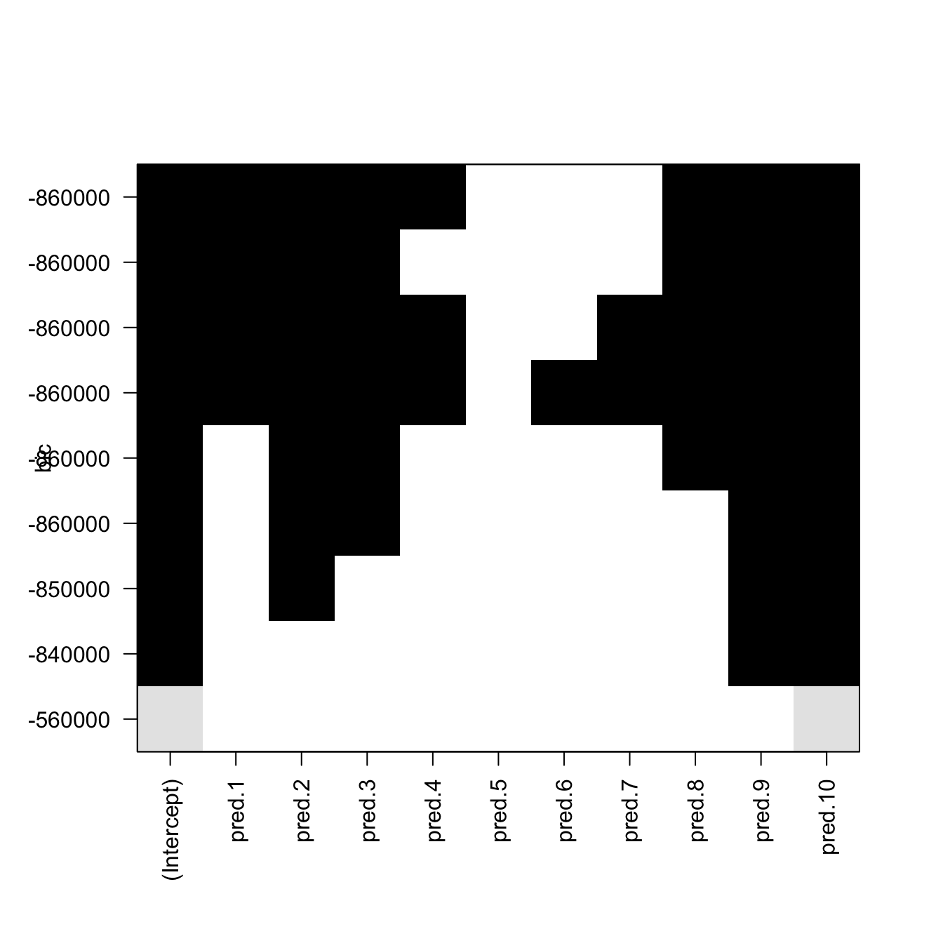
Figure 4.6: Best subsets for \(p=10\) predictors returned by leaps::regsubsets. The vertical axis indicates the sorting in terms of the BIC (the top positions contain the best models in terms of the BIC). White color indicates that the predictor is not included in the model and black that it is included. The \(p\) models obtained with the best subsets of \(1\leq r\leq p\) out of \(p\) predictors are displayed. Note that the vertical ordering does not necessarily coincide with \(r=1,\ldots,p\).
# Summarize (otherwise regsubsets's output is hard to decipher)
subs <- summary(reg)
subs
## Subset selection object
## 10 Variables  (and intercept)
##         Forced in Forced out
## pred.1      FALSE      FALSE
## pred.2      FALSE      FALSE
## pred.3      FALSE      FALSE
## pred.4      FALSE      FALSE
## pred.5      FALSE      FALSE
## pred.6      FALSE      FALSE
## pred.7      FALSE      FALSE
## pred.8      FALSE      FALSE
## pred.9      FALSE      FALSE
## pred.10     FALSE      FALSE
## 1 subsets of each size up to 9
## Selection Algorithm: exhaustive
##          pred.1 pred.2 pred.3 pred.4 pred.5 pred.6 pred.7 pred.8 pred.9 pred.10
## 1  ( 1 ) " "    " "    " "    " "    " "    " "    " "    " "    " "    "*"
## 2  ( 1 ) " "    " "    " "    " "    " "    " "    " "    " "    "*"    "*"
## 3  ( 1 ) " "    "*"    " "    " "    " "    " "    " "    " "    "*"    "*"
## 4  ( 1 ) " "    "*"    "*"    " "    " "    " "    " "    " "    "*"    "*"
## 5  ( 1 ) " "    "*"    "*"    " "    " "    " "    " "    "*"    "*"    "*"
## 6  ( 1 ) "*"    "*"    "*"    " "    " "    " "    " "    "*"    "*"    "*"
## 7  ( 1 ) "*"    "*"    "*"    "*"    " "    " "    " "    "*"    "*"    "*"
## 8  ( 1 ) "*"    "*"    "*"    "*"    " "    " "    "*"    "*"    "*"    "*"
## 9  ( 1 ) "*"    "*"    "*"    "*"    " "    "*"    "*"    "*"    "*"    "*"

# Lots of useful information
str(subs, 1)
## List of 8
##  $ which : logi [1:9, 1:11] TRUE TRUE TRUE TRUE TRUE TRUE ...
##   ..- attr(*, "dimnames")=List of 2
##  $ rsq   : num [1:9] 0.428 0.567 0.574 0.576 0.577 ...
##  $ rss   : num [1:9] 1352680 1023080 1006623 1003763 1001051 ...
##  $ adjr2 : num [1:9] 0.428 0.567 0.574 0.576 0.577 ...
##  $ cp    : num [1:9] 354480 24444 7968 5106 2392 ...
##  $ bic   : num [1:9] -558604 -837860 -854062 -856894 -859585 ...
##  $ outmat: chr [1:9, 1:10] " " " " " " " " ...
##   ..- attr(*, "dimnames")=List of 2
##  $ obj   :List of 27
##   ..- attr(*, "class")= chr "regsubsets"
##  - attr(*, "class")= chr "summary.regsubsets"

# Get the model with lowest BIC
subs$which
##   (Intercept) pred.1 pred.2 pred.3 pred.4 pred.5 pred.6 pred.7 pred.8 pred.9 pred.10
## 1        TRUE  FALSE  FALSE  FALSE  FALSE  FALSE  FALSE  FALSE  FALSE  FALSE    TRUE
## 2        TRUE  FALSE  FALSE  FALSE  FALSE  FALSE  FALSE  FALSE  FALSE   TRUE    TRUE
## 3        TRUE  FALSE   TRUE  FALSE  FALSE  FALSE  FALSE  FALSE  FALSE   TRUE    TRUE
## 4        TRUE  FALSE   TRUE   TRUE  FALSE  FALSE  FALSE  FALSE  FALSE   TRUE    TRUE
## 5        TRUE  FALSE   TRUE   TRUE  FALSE  FALSE  FALSE  FALSE   TRUE   TRUE    TRUE
## 6        TRUE   TRUE   TRUE   TRUE  FALSE  FALSE  FALSE  FALSE   TRUE   TRUE    TRUE
## 7        TRUE   TRUE   TRUE   TRUE   TRUE  FALSE  FALSE  FALSE   TRUE   TRUE    TRUE
## 8        TRUE   TRUE   TRUE   TRUE   TRUE  FALSE  FALSE   TRUE   TRUE   TRUE    TRUE
## 9        TRUE   TRUE   TRUE   TRUE   TRUE  FALSE   TRUE   TRUE   TRUE   TRUE    TRUE
subs$bic
## [1] -558603.7 -837859.9 -854062.3 -856893.8 -859585.3 -861936.5 -861939.3 -861932.3 -861918.6
subs$which[which.min(subs$bic), ]
## (Intercept)      pred.1      pred.2      pred.3      pred.4      pred.5      pred.6      pred.7      pred.8      pred.9
##        TRUE        TRUE        TRUE        TRUE        TRUE       FALSE       FALSE       FALSE        TRUE        TRUE
##     pred.10
##        TRUE

# Show the display in Figure 4.6
subs$which[order(subs$bic), ]
##   (Intercept) pred.1 pred.2 pred.3 pred.4 pred.5 pred.6 pred.7 pred.8 pred.9 pred.10
## 7        TRUE   TRUE   TRUE   TRUE   TRUE  FALSE  FALSE  FALSE   TRUE   TRUE    TRUE
## 6        TRUE   TRUE   TRUE   TRUE  FALSE  FALSE  FALSE  FALSE   TRUE   TRUE    TRUE
## 8        TRUE   TRUE   TRUE   TRUE   TRUE  FALSE  FALSE   TRUE   TRUE   TRUE    TRUE
## 9        TRUE   TRUE   TRUE   TRUE   TRUE  FALSE   TRUE   TRUE   TRUE   TRUE    TRUE
## 5        TRUE  FALSE   TRUE   TRUE  FALSE  FALSE  FALSE  FALSE   TRUE   TRUE    TRUE
## 4        TRUE  FALSE   TRUE   TRUE  FALSE  FALSE  FALSE  FALSE  FALSE   TRUE    TRUE
## 3        TRUE  FALSE   TRUE  FALSE  FALSE  FALSE  FALSE  FALSE  FALSE   TRUE    TRUE
## 2        TRUE  FALSE  FALSE  FALSE  FALSE  FALSE  FALSE  FALSE  FALSE   TRUE    TRUE
## 1        TRUE  FALSE  FALSE  FALSE  FALSE  FALSE  FALSE  FALSE  FALSE  FALSE    TRUE

# It also works with ordinary linear models and it is much faster and
# informative than stepAIC
reg <- leaps::regsubsets(resp ~ ., data = bigData1, nvmax = p,
                         method = "backward")
subs <- summary(reg)
subs$bic
##  [1] -558603.7 -837859.9 -854062.3 -856893.8 -859585.3 -861936.5 -861939.3 -861932.3 -861918.6 -861904.8
subs$which[which.min(subs$bic), ]
## (Intercept)      pred.1      pred.2      pred.3      pred.4      pred.5      pred.6      pred.7      pred.8      pred.9
##        TRUE        TRUE        TRUE        TRUE        TRUE       FALSE       FALSE       FALSE        TRUE        TRUE
##     pred.10
##        TRUE

# Compare it with stepAIC
MASS::stepAIC(lm(resp ~ ., data = bigData1), trace = 0,
              direction = "backward", k = log(n))
##
## Call:
## lm(formula = resp ~ pred.1 + pred.2 + pred.3 + pred.4 + pred.8 +
##     pred.9 + pred.10, data = bigData1)
##
## Coefficients:
## (Intercept)       pred.1       pred.2       pred.3       pred.4       pred.8       pred.9      pred.10
##    1.002141    -0.973201    -0.286626    -0.053487    -0.004074     0.052076     0.284038     0.986651
Finally, let’s see an example on how to fit a linear model to a large dataset that does not fit in the RAM of most regular laptops. Imagine that you want to regress a response \(Y\) into a set of \(p=10\) predictors and the sample size is \(n=10^8.\) Merely storing the response and the predictors will take up to \(8.2\) GB in RAM:
# Size of the response
print(object.size(rnorm(1e6)) * 1e2, units = "GB")
## 0.7 Gb

# Size of the predictors
print(object.size(rnorm(1e6)) * 1e2 * 10, units = "GB")
## 7.5 Gb
In addition to this, if lm was called, it will return the residuals, effects, and fitted.values slots (all vectors of length \(n,\) hence \(0.7 \times 3=2.1\) GB more). It will also return the qr decomposition of the design matrix and the model matrix (both are \(n\times (p + 1)\) matrices, so another \(8.2\times 2=16.4\) GB more). The final lm object will thus be at the very least, of size \(18.5\) GB. Clearly, this is not a very memory-friendly procedure.
A possible approach is to split the dataset and perform updates of the model in chunks of reasonable size. The next code provides a template for such approach using biglm and update.
# Linear regression with n = 10^8 and p = 10
n <- 10^8
p <- 10
beta <- seq(-1, 1, length.out = p)^5

# Number of chunks for splitting the dataset
nChunks <- 1e3
nSmall <- n / nChunks

# Simulates reading the first chunk of data
set.seed(12345)
x <- matrix(rnorm(nSmall * p), nrow = nSmall, ncol = p)
x[, p] <- 2 * x[, 1] + rnorm(nSmall, sd = 0.1)
x[, p - 1] <- 2 - x[, 2] + rnorm(nSmall, sd = 0.5)
y <- 1 + x %*% beta + rnorm(nSmall)

# First fit
bigMod <- biglm::biglm(y ~ x, data = data.frame(y, x))

# Update fit
# pb <- txtProgressBar(style = 3)
for (i in 2:nChunks) {

  # Simulates reading the i-th chunk of data
  set.seed(12345 + i)
  x <- matrix(rnorm(nSmall * p), nrow = nSmall, ncol = p)
  x[, p] <- 2 * x[, 1] + rnorm(nSmall, sd = 0.1)
  x[, p - 1] <- 2 - x[, 2] + rnorm(nSmall, sd = 0.5)
  y <- 1 + x %*% beta + rnorm(nSmall)

  # Update the fit
  bigMod <- update(bigMod, moredata = data.frame(y, x))

  # Progress
  # setTxtProgressBar(pb = pb, value = i / nChunks)

}

# Final model
summary(bigMod)
## Large data regression model: biglm::biglm(y ~ x, data = data.frame(y, x))
## Sample size =  100000000
##                Coef    (95%     CI)    SE      p
## (Intercept)  1.0003  0.9995  1.0011 4e-04 0.0000
## x1          -1.0015 -1.0055 -0.9975 2e-03 0.0000
## x2          -0.2847 -0.2852 -0.2843 2e-04 0.0000
## x3          -0.0531 -0.0533 -0.0529 1e-04 0.0000
## x4          -0.0041 -0.0043 -0.0039 1e-04 0.0000
## x5           0.0002  0.0000  0.0004 1e-04 0.0760
## x6          -0.0001 -0.0003  0.0001 1e-04 0.2201
## x7           0.0041  0.0039  0.0043 1e-04 0.0000
## x8           0.0529  0.0527  0.0531 1e-04 0.0000
## x9           0.2844  0.2840  0.2848 2e-04 0.0000
## x10          1.0007  0.9987  1.0027 1e-03 0.0000
print(object.size(bigMod), units = "KB")
## 7.8 Kbsummary of a biglm object yields slightly different significances for the coefficients than those of lm. The reason is that biglm employs \(\mathcal{N}(0,1)\)-approximations for the distributions of the \(t\)-tests instead of the exact \(t_{n-1}\) distribution. Obviously, if \(n\) is large, the differences are inappreciable.
References
The QR decomposition of the matrix \(\mathbf{X}\) of size \(n\times m\) is \(\mathbf{X}=\mathbf{Q}\mathbf{R}\) such that \(\mathbf{Q}\) is an \(n\times n\) orthogonal matrix and \(\mathbf{R}\) is an \(n\times m\) upper triangular matrix. This factorization is commonly used in numerical analysis for solving linear systems.↩︎
Not really exhaustive: the method behind it, due to Furnival and Wilson (1974), employs an ingenious branch and bound algorithm to remove most of the non-interesting models.↩︎