6.1 Nonparametric density estimation

In order to introduce a nonparametric estimator for the regression function $m,$ we need to introduce first a nonparametric estimator for the density of the predictor $X.$ This estimator is aimed to estimate $f,$ the density of $X,$ from a sample $X_1,\ldots,X_n$ without assuming any specific form for $f.$ This is, without assuming, e.g., that the data is normally distributed.

6.1.1 Histogram and moving histogram

The simplest method to estimate a density $f$ from an iid sample $X_1,\ldots,X_n$ is the histogram. From an analytical point of view, the idea is to aggregate the data in intervals of the form $[x_0,x_0+h)$ and then use their relative frequency to approximate the density at $x\in[x_0,x_0+h),$ $f(x),$ by the estimate of

\[\begin{align*} f(x_0)&=F'(x_0)\\ &=\lim_{h\to0^+}\frac{F(x_0+h)-F(x_0)}{h}\\ &=\lim_{h\to0^+}\frac{\mathbb{P}[x_0<X< x_0+h]}{h}. \end{align*}\]

More precisely, given an origin $t_0$ and a bandwidth $h>0,$ the histogram builds a piecewise constant function in the intervals $\{B_k:=[t_{k},t_{k+1}):t_k=t_0+hk,k\in\mathbb{Z}\}$ by counting the number of sample points inside each of them. These constant-length intervals are also called bins. The fact they have constant length $h$ is important, since it allows to standardize by $h$ in order to have relative frequencies per length¹⁸⁷ in the bins. The histogram at a point $x$ is defined as

\[\begin{align} \hat{f}_\mathrm{H}(x;t_0,h):=\frac{1}{nh}\sum_{i=1}^n1_{\{X_i\in B_k:x\in B_k\}}. \tag{6.1} \end{align}\]

Equivalently, if we denote the number of points in $B_k$ as $v_k,$ then the histogram is $\hat{f}_\mathrm{H}(x;t_0,h)=\frac{v_k}{nh}$ if $x\in B_k$ for $k\in\mathbb{Z}.$

The computation of histograms is straightforward in R. As an example, we consider the faithful dataset, which contains the duration of the eruption and the waiting time between eruptions for the Old Faithful geyser in Yellowstone National Park (USA).

# Duration of eruption
faithE <- faithful$eruptions

# Default histogram: automatically chooses bins and uses absolute frequencies
histo <- hist(faithE)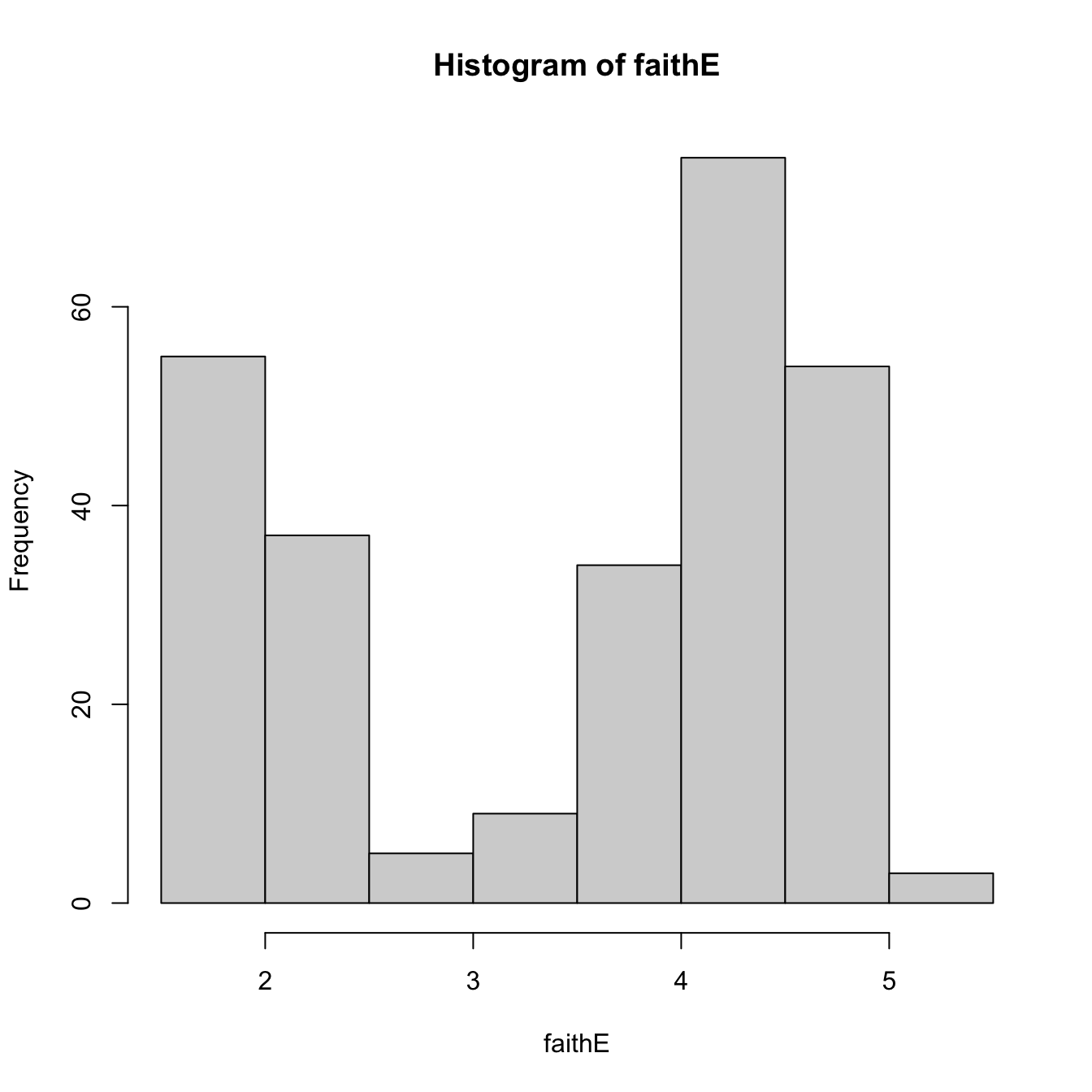


# Bins and bin counts
histo$breaks # Bk's
## [1] 1.5 2.0 2.5 3.0 3.5 4.0 4.5 5.0 5.5
histo$counts # vk's
## [1] 55 37  5  9 34 75 54  3

# With relative frequencies
hist(faithE, probability = TRUE)


# Choosing the breaks
t0 <- min(faithE)
h <- 0.25
Bk <- seq(t0, max(faithE), by = h)
hist(faithE, probability = TRUE, breaks = Bk)
rug(faithE) # The sample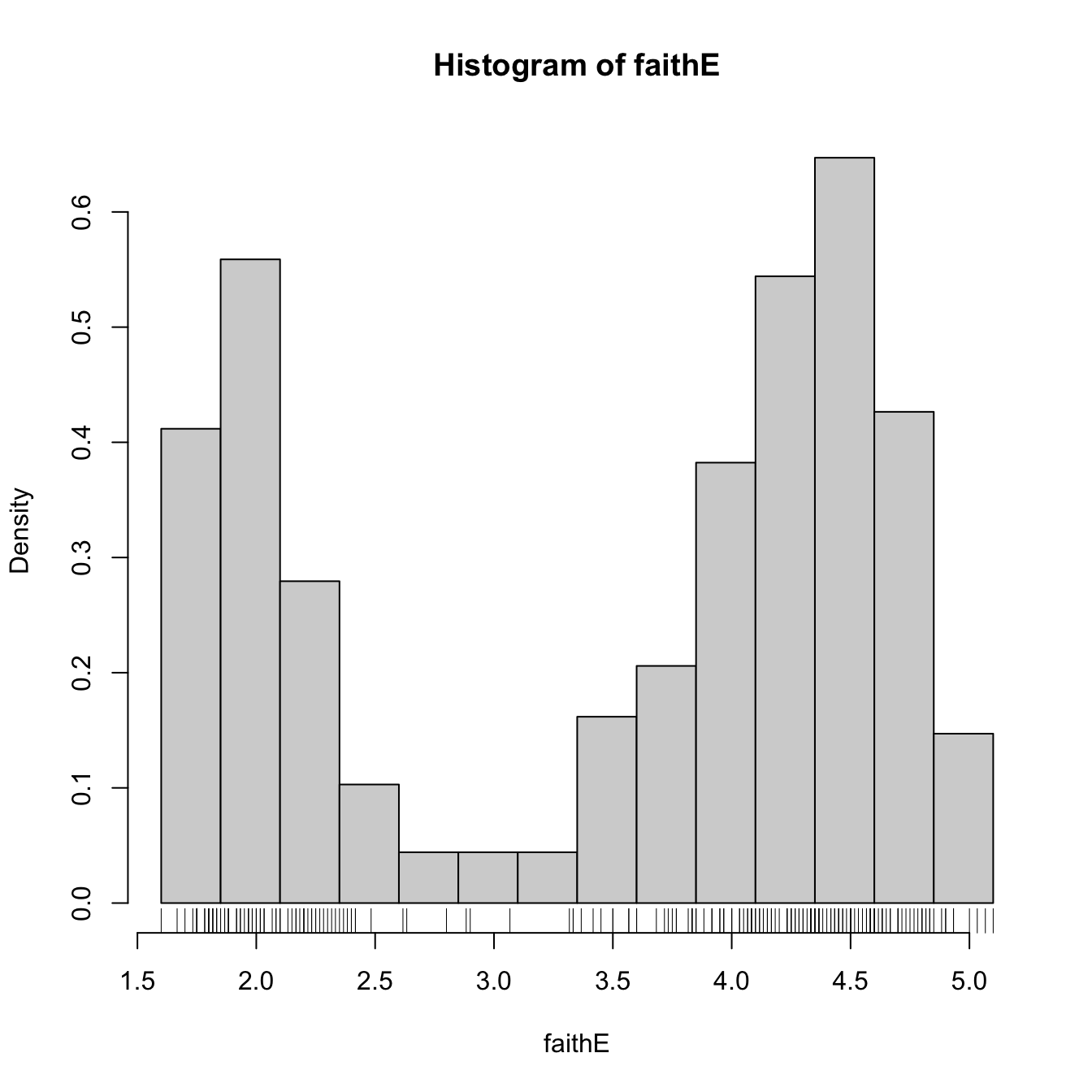

Recall that the shape of the histogram depends on:

$t_0,$ since the separation between bins happens at $t_0k,$ $k\in\mathbb{Z};$
$h,$ which controls the bin size and the effective number of bins for aggregating the sample.

We focus first on exploring the dependence on $t_0$ with the next example, as it serves for motivating the next density estimator.

# Uniform sample
set.seed(1234567)
u <- runif(n = 100)

# t0 = 0, h = 0.2
Bk1 <- seq(0, 1, by = 0.2)

# t0 = -0.1, h = 0.2
Bk2 <- seq(-0.1, 1.1, by = 0.2)

# Comparison
par(mfrow = 1:2)
hist(u, probability = TRUE, breaks = Bk1, ylim = c(0, 1.5),
     main = "t0 = 0, h = 0.2")
rug(u)
abline(h = 1, col = 2)
hist(u, probability = TRUE, breaks = Bk2, ylim = c(0, 1.5),
     main = "t0 = -0.1, h = 0.2")
rug(u)
abline(h = 1, col = 2)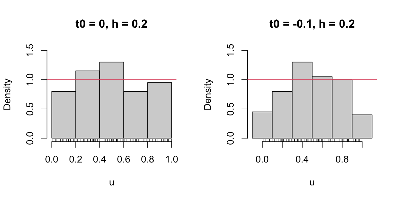

$The dependence of the histogram on the origin $t_0$.$

Figure 6.1: The dependence of the histogram on the origin $t_0$.

Clearly, this dependence is undesirable, as it is prone to change notably the estimation of $f$ using the same data. An alternative to avoid the dependence on $t_0$ is the moving histogram or naive density estimator. The idea is to aggregate the sample $X_1,\ldots,X_n$ in intervals of the form $(x-h, x+h)$ and then use its relative frequency in $(x-h,x+h)$ to approximate the density at $x,$ which can be written as

\[\begin{align*} f(x)&=F'(x)\\ &=\lim_{h\to0^+}\frac{F(x+h)-F(x-h)}{2h}\\ &=\lim_{h\to0^+}\frac{\mathbb{P}[x-h<X<x+h]}{2h}. \end{align*}\]

Recall the differences with the histogram: the intervals depend on the evaluation point $x$ and are centered about it. That allows to directly estimate $f(x)$ (without the proxy $f(x_0)$) by an estimate of the symmetric derivative.

Given a bandwidth $h>0,$ the naive density estimator builds a piecewise constant function by considering the relative frequency of $X_1,\ldots,X_n$ inside $(x-h,x+h)\;$¹⁸⁸:

\[\begin{align} \hat{f}_\mathrm{N}(x;h):=\frac{1}{2nh}\sum_{i=1}^n1_{\{x-h<X_i<x+h\}}. \tag{6.2} \end{align}\]

The analysis of $\hat{f}_\mathrm{N}(x;h)$ as a random variable follows from realizing that

\[\begin{align*} \sum_{i=1}^n1_{\{x-h<X_i<x+h\}}\sim \mathrm{B}(n,p_{x,h}) \end{align*}\]

where

\[\begin{align*} p_{x,h}:=\mathbb{P}[x-h<X<x+h]=F(x+h)-F(x-h). \end{align*}\]

Therefore, employing the bias and variance expressions of a binomial¹⁸⁹, it follows:

\[\begin{align*} \mathbb{E}[\hat{f}_\mathrm{N}(x;h)]=&\,\frac{F(x+h)-F(x-h)}{2h},\\ \mathbb{V}\mathrm{ar}[\hat{f}_\mathrm{N}(x;h)]=&\,\frac{F(x+h)-F(x-h)}{4nh^2}\\ &-\frac{(F(x+h)-F(x-h))^2}{4nh^2}. \end{align*}\]

These two results provide very interesting insights on the effect of $h$ on the moving histogram:

If $h\to0,$ then $\mathbb{E}[\hat{f}_\mathrm{N}(x;h)]\to f(x)$ and (6.2) is an asymptotically unbiased estimator of $f(x).$ However, if $h\to0,$ the variance explodes: $\mathbb{V}\mathrm{ar}[\hat{f}_\mathrm{N}(x;h)]\approx \frac{f(x)}{2nh}-\frac{f(x)^2}{n}\to\infty.$
If $h\to\infty,$ then both $\mathbb{E}[\hat{f}_\mathrm{N}(x;h)]\to 0$ and $\mathbb{V}\mathrm{ar}[\hat{f}_\mathrm{N}(x;h)]\to0.$ Therefore, the variance shrinks to zero but the bias grows.
If $nh\to\infty\;$¹⁹⁰, then the variance shrinks to zero. If, in addition, $h\to0,$ the bias also shrinks to zero. So both the bias and the variance are reduced if $n\to\infty,$ $h\to0,$ and $nh\to\infty,$ simultaneously.

The animation in Figure 6.2 illustrates the previous points and gives insight on how the performance of (6.2) varies with $h.$

Figure 6.2: Bias and variance for the moving histogram. The animation shows how for small bandwidths the bias of $\hat{f}_\mathrm{N}(x;h)$ on estimating $f(x)$ is small, but the variance is high, and how for large bandwidths the bias is large and the variance is small. The variance is represented by the asymptotic $95\%$ confidence intervals for $\hat{f}_\mathrm{N}(x;h).$ Recall how the variance of $\hat{f}_\mathrm{N}(x;h)$ is (almost) proportional to $f(x).$ Application also available here.

The estimator (6.2) poses an interesting question:

Why giving the same weight to all $X_1,\ldots,X_n$ in $(x-h, x+h)$ for estimating $f(x)$?

We are estimating $f(x)=F'(x)$ by estimating $\frac{F(x+h)-F(x-h)}{2h}$ through the relative frequency of $X_1,\ldots,X_n$ in the interval $(x-h,x+h).$ Should not be the data points closer to $x$ more important than the ones further away? The answer to this question shows that (6.2) is indeed a particular case of a wider class of density estimators.

6.1.2 Kernel density estimation

The moving histogram (6.2) can be equivalently written as

\[\begin{align} \hat{f}_\mathrm{N}(x;h)&=\frac{1}{nh}\sum_{i=1}^n\frac{1}{2}1_{\left\{-1<\frac{x-X_i}{h}<1\right\}}\nonumber\\ &=\frac{1}{nh}\sum_{i=1}^nK\left(\frac{x-X_i}{h}\right), \tag{6.3} \end{align}\]

with $K(z)=\frac{1}{2}1_{\{-1<z<1\}}.$ Interestingly, $K$ is a uniform density in $(-1,1).$ This means that, when approximating

\[\begin{align*} \mathbb{P}[x-h<X<x+h]=\mathbb{P}\left[-1<\frac{x-X}{h}<1\right] \end{align*}\]

by (6.3), we give equal weight to all the points $X_1,\ldots,X_n.$ The generalization of (6.3) is now obvious: replace $K$ by an arbitrary density. Then $K$ is known as a kernel: a density with certain regularity that is (typically) symmetric and unimodal at $0.$ This generalization provides the definition of kernel density estimator¹⁹¹ (kde):

\[\begin{align} \hat{f}(x;h):=\frac{1}{nh}\sum_{i=1}^nK\left(\frac{x-X_i}{h}\right). \tag{6.4} \end{align}\]

A common notation is $K_h(z):=\frac{1}{h}K\left(\frac{z}{h}\right),$ so the kde can be compactly written as $\hat{f}(x;h)=\frac{1}{n}\sum_{i=1}^nK_h(x-X_i).$

It is useful to recall (6.4) with the normal kernel. If that is the case, then $K_h(x-X_i)=\phi(x;X_i,h^2)=\phi(x-X_i;0,h^2)$ (denoted simply as $\phi(x-X_i;h^2)$) and the kernel is the density of a $\mathcal{N}(X_i,h^2).$ Thus the bandwidth $h$ can be thought of as the standard deviation of a normal density whose mean is $X_i$ and the kde (6.4) as a data-driven mixture of those densities. Figure 6.3 illustrates the construction of the kde, and the bandwidth and kernel effects.

Figure 6.3: Construction of the kernel density estimator. The animation shows how the bandwidth and kernel affect the density estimate, and how the kernels are rescaled densities with modes at the data points. Application available here.

Several types of kernels are possible. The most popular is the normal kernel $K(z)=\phi(z),$ although the Epanechnikov kernel, $K(z)=\frac{3}{4}(1-z^2)1_{\{|z|<1\}},$ is the most efficient¹⁹². The rectangular kernel $K(z)=\frac{1}{2}1_{\{|z|<1\}}$ yields the moving histogram as a particular case. The kde inherits the smoothness properties of the kernel. That means, e.g., that (6.4) with a normal kernel is infinitely differentiable. But, with an Epanechnikov kernel, (6.4) is not differentiable, and, with a rectangular kernel, the kde is not even continuous. However, if a certain smoothness is guaranteed (continuity at least), then the choice of the kernel has little importance in practice (at least compared with the choice of the bandwidth $h$).

The computation of the kde in R is done through the density function. The function automatically chooses the bandwidth $h$ using a data-driven criterion¹⁹³.

# Sample 100 points from a N(0, 1)
set.seed(1234567)
samp <- rnorm(n = 100, mean = 0, sd = 1)

# Quickly compute a kernel density estimator and plot the density object
# Automatically chooses bandwidth and uses normal kernel
plot(density(x = samp))

# Select a particular bandwidth (0.5) and kernel (Epanechnikov)
lines(density(x = samp, bw = 0.5, kernel = "epanechnikov"), col = 2)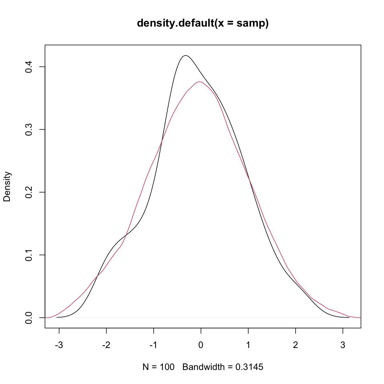

# density() automatically chooses the interval for plotting the kernel density
# estimator (observe that the black line goes to roughly between -3 and 3)

# This can be tuned using "from" and "to"
plot(density(x = samp, from = -4, to = 4), xlim = c(-5, 5))


# The density object is a list
kde <- density(x = samp, from = -5, to = 5, n = 1024)
str(kde)
## List of 7
##  $ x        : num [1:1024] -5 -4.99 -4.98 -4.97 -4.96 ...
##  $ y        : num [1:1024] 4.91e-17 2.97e-17 1.86e-17 2.53e-17 3.43e-17 ...
##  $ bw       : num 0.315
##  $ n        : int 100
##  $ call     : language density.default(x = samp, n = 1024, from = -5, to = 5)
##  $ data.name: chr "samp"
##  $ has.na   : logi FALSE
##  - attr(*, "class")= chr "density"
# Note that the evaluation grid "x"" is not directly controlled, only through
# "from, "to", and "n" (better use powers of 2). This is because, internally,
# kde employs an efficient Fast Fourier Transform on grids of size 2^m

# Plotting the returned values of the kde
plot(kde$x, kde$y, type = "l")
curve(dnorm(x), col = 2, add = TRUE) # True density
rug(samp)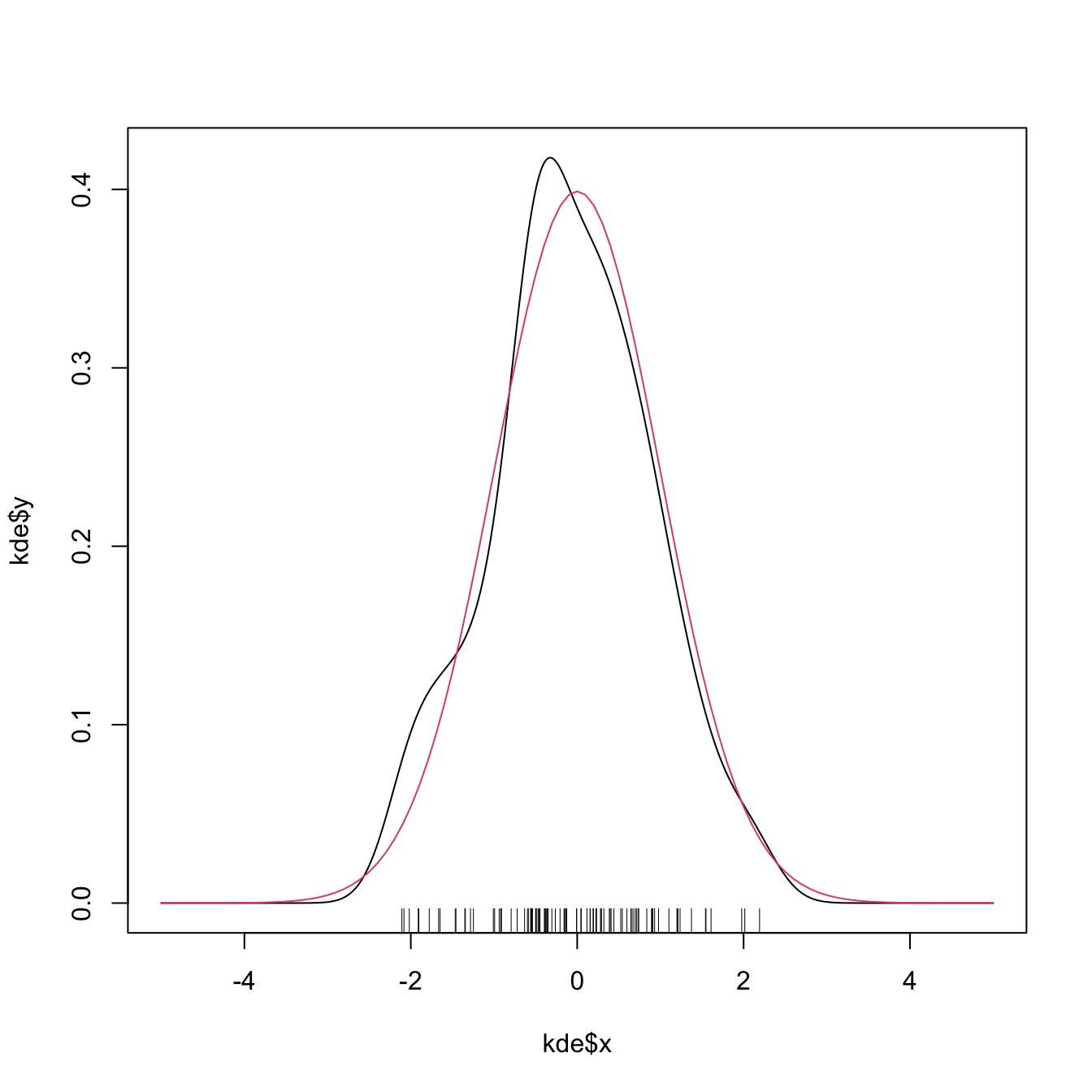

Load the dataset faithful. Then:

Estimate and plot the density of faithful$eruptions.
Create a new plot and superimpose different density estimations with bandwidths equal to $0.1,$ $0.5,$ and $1.$
Get the density estimate at exactly the point $x=3.1$ using $h=0.15$ and the Epanechnikov kernel.

6.1.3 Bandwidth selection

The kde critically depends on the employed bandwidth; hence objective and automatic bandwidth selectors that attempt to minimize the estimation error of the target density $f$ are required to properly apply a kde in practice.

A global, rather than local, error criterion for the kde is the Integrated Squared Error (ISE):

\[\begin{align*} \mathrm{ISE}[\hat{f}(\cdot;h)]:=\int (\hat{f}(x;h)-f(x))^2\,\mathrm{d}x. \end{align*}\]

The ISE is a random quantity, since it depends directly on the sample $X_1,\ldots,X_n.$ As a consequence, looking for an optimal-ISE bandwidth is a hard task, since the optimality is dependent on the sample itself (not only on $f$ and $n$). To avoid this problematic, it is usual to compute the Mean Integrated Squared Error (MISE):

\[\begin{align*} \mathrm{MISE}[\hat{f}(\cdot;h)]:=&\,\mathbb{E}\left[\mathrm{ISE}[\hat{f}(\cdot;h)]\right]\\ =&\,\int \mathbb{E}\left[(\hat{f}(x;h)-f(x))^2\right]\,\mathrm{d}x\\ =&\,\int \mathrm{MSE}[\hat{f}(x;h)]\,\mathrm{d}x. \end{align*}\]

Once the MISE is set as the error criterion to be minimized, our aim is to find

\[\begin{align*} h_\mathrm{MISE}:=\arg\min_{h>0}\mathrm{MISE}[\hat{f}(\cdot;h)]. \end{align*}\]

For that purpose, we need an explicit expression of the MISE that we can attempt to minimize. An asymptotic expansion can be derived when $h\to0$ and $nh\to\infty,$ resulting in

\[\begin{align} \mathrm{MISE}[\hat{f}(\cdot;h)]\approx\mathrm{AMISE}[\hat{f}(\cdot;h)]:=\frac{1}{4}\mu^2_2(K)R(f'')h^4+\frac{R(K)}{nh},\tag{6.5} \end{align}\]

where $\mu_2(K):=\int z^2K(z)\,\mathrm{d}z$ and $R(g):=\int g(x)^2\,\mathrm{d}x.$ The AMISE stands for Asymptotic MISE and, due to its closed expression, it allows to obtain a bandwidth that minimizes it:¹⁹⁴

\[\begin{align} h_\mathrm{AMISE}=\left[\frac{R(K)}{\mu_2^2(K)R(f'')n}\right]^{1/5}.\tag{6.6} \end{align}\]

Unfortunately, the AMISE bandwidth depends on $R(f'')=\int(f''(x))^2\,\mathrm{d}x,$ which measures the curvature of the unknown density $f.$ As a consequence, it cannot be readily applied in practice!

Plug-in selectors

A simple solution to turn (6.6) into something computable is to estimate $R(f'')$ by assuming that $f$ is the density of a $\mathcal{N}(\mu,\sigma^2),$ and then plug-in the form of the curvature for such density:

\[\begin{align*} R(\phi''(\cdot;\mu,\sigma^2))=\frac{3}{8\pi^{1/2}\sigma^5}. \end{align*}\]

While doing so, we approximate the curvature of an arbitrary density by means of the curvature of a normal and we have that

\[\begin{align*} h_\mathrm{AMISE}=\left[\frac{8\pi^{1/2}R(K)}{3\mu_2^2(K)n}\right]^{1/5}\sigma. \end{align*}\]

Interestingly, the bandwidth is directly proportional to the standard deviation of the target density. Replacing $\sigma$ by an estimate yields the normal scale bandwidth selector, which we denote by $\hat{h}_\mathrm{NS}$ to emphasize its randomness:

\[\begin{align*} \hat{h}_\mathrm{NS}=\left[\frac{8\pi^{1/2}R(K)}{3\mu_2^2(K)n}\right]^{1/5}\hat\sigma. \end{align*}\]

The estimate $\hat\sigma$ can be chosen as the standard deviation $s,$ or, in order to avoid the effects of potential outliers, as the standardized interquantile range

\[\begin{align*} \hat \sigma_{\mathrm{IQR}}:=\frac{X_{([0.75n])}-X_{([0.25n])}}{\Phi^{-1}(0.75)-\Phi^{-1}(0.25)} \end{align*}\]

or as

\[\begin{align} \hat\sigma=\min(s,\hat \sigma_{\mathrm{IQR}}). \tag{6.7} \end{align}\]

When combined with a normal kernel, for which $\mu_2(K)=1$ and $R(K)=\frac{1}{2\sqrt{\pi}},$ this particularization of $\hat{h}_{\mathrm{NS}}$ gives the famous rule-of-thumb for bandwidth selection:

\[\begin{align*} \hat{h}_\mathrm{RT}=\left(\frac{4}{3}\right)^{1/5}n^{-1/5}\hat\sigma\approx1.06n^{-1/5}\hat\sigma. \end{align*}\]

$\hat{h}_{\mathrm{RT}}$ is implemented in R through the function bw.nrd¹⁹⁵.

# Data
set.seed(667478)
n <- 100
x <- rnorm(n)

# Rule-of-thumb
bw.nrd(x = x)
## [1] 0.4040319
# bwd.nrd employs 1.34 as an approximation for diff(qnorm(c(0.25, 0.75)))

# Same as
iqr <- diff(quantile(x, c(0.25, 0.75))) / diff(qnorm(c(0.25, 0.75)))
1.06 * n^(-1/5) * min(sd(x), iqr)
## [1] 0.4040319

The rule-of-thumb is an example of a zero-stage plug-in selector, a terminology which lays on the fact that $R(f'')$ was estimated by plugging-in a parametric estimation at “the very first moment a quantity that depends on $f$ appears”. We could have opted to estimate $R(f'')$ nonparametrically, in a certain optimal way, and then plug-in the estimate into into $h_\mathrm{AMISE}.$ The important catch lies on the optimal estimation of $R(f'')$ : it requires the knowledge of $R\big(f^{(4)}\big)$! What $\ell$-stage plug-in selectors do is to iterate these steps $\ell$ times and finally plug-in a normal estimate of the unknown $R\big(f^{(2\ell)}\big)\;$¹⁹⁶.

Typically, two stages are considered a good trade-off between bias (mitigated when $\ell$ increases) and variance (augments with $\ell$) of the plug-in selector. This is the method proposed by Sheather and Jones (1991), yielding what we call the Direct Plug-In (DPI). The DPI selector is implemented in R through the function bw.SJ (use method = "dpi"). An alternative and faster implementation is ks::hpi, which also for more flexibility and has a somehow more detailed documentation.

# Data
set.seed(672641)
x <- rnorm(100)

# DPI selector
bw.SJ(x = x, method = "dpi")
## [1] 0.5006905

# Similar to
ks::hpi(x) # Default is two-stages
## [1] 0.4999456

Cross-validation

We turn now our attention to a different philosophy of bandwidth estimation. Instead of trying to minimize the AMISE by plugging-in estimates for the unknown curvature term, we directly attempt to minimize the MISE by using the sample twice: one for computing the kde and other for evaluating its performance on estimating $f.$ To avoid the clear dependence on the sample, we do the evaluation in a cross-validatory way: the data used for computing the kde is not used for its evaluation.

We begin by expanding the square in the MISE expression:

\[\begin{align*} \mathrm{MISE}[\hat{f}(\cdot;h)]=&\,\mathbb{E}\left[\int (\hat{f}(x;h)-f(x))^2\,\mathrm{d}x\right]\\ =&\,\mathbb{E}\left[\int \hat{f}(x;h)^2\,\mathrm{d}x\right]-2\mathbb{E}\left[\int \hat{f}(x;h)f(x)\,\mathrm{d}x\right]\\ &+\int f(x)^2\,\mathrm{d}x. \end{align*}\]

Since the last term does not depend on $h,$ minimizing $\mathrm{MISE}[\hat{f}(\cdot;h)]$ is equivalent to minimizing

\[\begin{align*} \mathbb{E}\left[\int \hat{f}(x;h)^2\,\mathrm{d}x\right]-2\mathbb{E}\left[\int \hat{f}(x;h)f(x)\,\mathrm{d}x\right]. \end{align*}\]

This quantity is unknown, but it can be estimated unbiasedly by

\[\begin{align} \mathrm{LSCV}(h):=\int\hat{f}(x;h)^2\,\mathrm{d}x-2n^{-1}\sum_{i=1}^n\hat{f}_{-i}(X_i;h),\tag{6.8} \end{align}\]

where $\hat{f}_{-i}(\cdot;h)$ is the leave-one-out kde and is based on the sample with the $X_i$ removed:

\[\begin{align*} \hat{f}_{-i}(x;h)=\frac{1}{n-1}\sum_{\substack{j=1\\j\neq i}}^n K_h(x-X_j). \end{align*}\]

The Least Squares Cross-Validation (LSCV) selector, also denoted Unbiased Cross-Validation (UCV) selector, is defined as

\[\begin{align*} \hat{h}_\mathrm{LSCV}:=\arg\min_{h>0}\mathrm{LSCV}(h). \end{align*}\]

Numerical optimization is required for obtaining $\hat{h}_\mathrm{LSCV},$ contrary to the previous plug-in selectors, and there is little control on the shape of the objective function.

Numerical optimization of the (6.8) can be challenging. In practice, several local minima are possible, and the roughness of the objective function can vary notably depending on $n$ and $f.$ As a consequence, optimization routines may get trapped in spurious solutions. To be on the safe side, it is advisable to check the solution by plotting $\mathrm{LSCV}(h)$ for a range of $h,$ or to perform an exhaustive search in a bandwidth grid: $\hat{h}_\mathrm{LSCV}\approx\arg\min_{h_1,\ldots,h_G}\mathrm{LSCV}(h).$

$\hat{h}_{\mathrm{LSCV}}$ is implemented in R through the function bw.ucv. bw.ucv uses optimize, which is quite sensible to the selection of the search interval¹⁹⁷. Therefore, some care is needed and that is why the bw.ucv.mod function is presented.

# Data
set.seed(123456)
x <- rnorm(100)

# UCV gives a warning
bw.ucv(x = x)
## [1] 0.4499177

# Extend search interval
bw.ucv(x = x, lower = 0.01, upper = 1)
## [1] 0.5482419

# bw.ucv.mod replaces the optimization routine of bw.ucv by an exhaustive
# search on "h.grid" (chosen adaptatively from the sample) and optionally
# plots the LSCV curve with "plot.cv"
bw.ucv.mod <- function(x, nb = 1000L,
                       h.grid = diff(range(x)) * (seq(0.1, 1, l = 200))^2,
                       plot.cv = FALSE) {
  if ((n <- length(x)) < 2L)
    stop("need at least 2 data points")
  n <- as.integer(n)
  if (is.na(n))
    stop("invalid length(x)")
  if (!is.numeric(x))
    stop("invalid 'x'")
  nb <- as.integer(nb)
  if (is.na(nb) || nb <= 0L)
    stop("invalid 'nb'")
  storage.mode(x) <- "double"
  hmax <- 1.144 * sqrt(var(x)) * n^(-1/5)
  Z <- .Call(stats:::C_bw_den, nb, x)
  d <- Z[[1L]]
  cnt <- Z[[2L]]
  fucv <- function(h) .Call(stats:::C_bw_ucv, n, d, cnt, h)
  ## Original
  # h <- optimize(fucv, c(lower, upper), tol = tol)$minimum
  # if (h < lower + tol | h > upper - tol)
  #   warning("minimum occurred at one end of the range")
  ## Modification
  obj <- sapply(h.grid, function(h) fucv(h))
  h <- h.grid[which.min(obj)]
  if (plot.cv) {
    plot(h.grid, obj, type = "o")
    rug(h.grid)
    abline(v = h, col = 2, lwd = 2)
  }
  h
}

# Compute the bandwidth and plot the LSCV curve
bw.ucv.mod(x = x, plot.cv = TRUE)
## [1] 0.5431732

# We can compare with the default bw.ucv output
abline(v = bw.ucv(x = x), col = 3)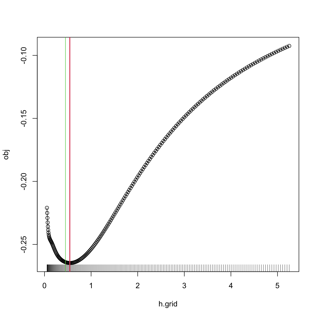

The next cross-validation selector is based on Biased Cross-Validation (BCV). The BCV selector presents a hybrid strategy that combines plug-in and cross-validation ideas. It starts by considering the AMISE expression in (6.5) and then plugs-in an estimate for $R(f'')$ based on a modification of $R(\hat{f}''(\cdot;h)).$ The appealing property of $\hat{h}_\mathrm{BCV}$ is that it has a considerably smaller variance compared to $\hat{h}_\mathrm{LSCV}.$ This reduction in variance comes at the price of an increased bias, which tends to make $\hat{h}_\mathrm{BCV}$ larger than $h_\mathrm{MISE}.$

$\hat{h}_{\mathrm{BCV}}$ is implemented in R through the function bw.bcv. Again, bw.bcv uses optimize so the bw.bcv.mod function is presented to have better guarantees on finding the adequate minimum.¹⁹⁸

# Data
set.seed(123456)
x <- rnorm(100)

# BCV gives a warning
bw.bcv(x = x)
## [1] 0.4500924

# Extend search interval
args(bw.bcv)
## function (x, nb = 1000L, lower = 0.1 * hmax, upper = hmax, tol = 0.1 * 
##     lower) 
## NULL
bw.bcv(x = x, lower = 0.01, upper = 1)
## [1] 0.5070129

# bw.bcv.mod replaces the optimization routine of bw.bcv by an exhaustive
# search on "h.grid" (chosen adaptatively from the sample) and optionally
# plots the BCV curve with "plot.cv"
bw.bcv.mod <- function(x, nb = 1000L,
                       h.grid = diff(range(x)) * (seq(0.1, 1, l = 200))^2,
                       plot.cv = FALSE) {
  if ((n <- length(x)) < 2L)
    stop("need at least 2 data points")
  n <- as.integer(n)
  if (is.na(n))
    stop("invalid length(x)")
  if (!is.numeric(x))
    stop("invalid 'x'")
  nb <- as.integer(nb)
  if (is.na(nb) || nb <= 0L)
    stop("invalid 'nb'")
  storage.mode(x) <- "double"
  hmax <- 1.144 * sqrt(var(x)) * n^(-1/5)
  Z <- .Call(stats:::C_bw_den, nb, x)
  d <- Z[[1L]]
  cnt <- Z[[2L]]
  fbcv <- function(h) .Call(stats:::C_bw_bcv, n, d, cnt, h)
  ## Original code
  # h <- optimize(fbcv, c(lower, upper), tol = tol)$minimum
  # if (h < lower + tol | h > upper - tol)
  #   warning("minimum occurred at one end of the range")
  ## Modification
  obj <- sapply(h.grid, function(h) fbcv(h))
  h <- h.grid[which.min(obj)]
  if (plot.cv) {
    plot(h.grid, obj, type = "o")
    rug(h.grid)
    abline(v = h, col = 2, lwd = 2)
  }
  h
}

# Compute the bandwidth and plot the BCV curve
bw.bcv.mod(x = x, plot.cv = TRUE)
## [1] 0.5130493

# We can compare with the default bw.bcv output
abline(v = bw.bcv(x = x), col = 3)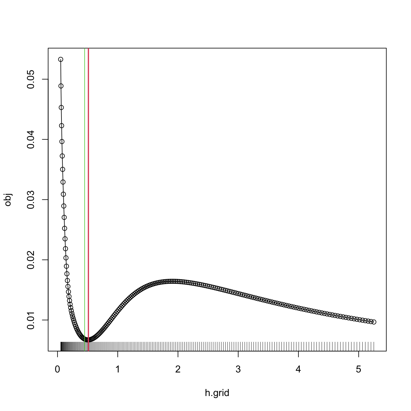

Comparison of bandwidth selectors

Despite it is possible to compare theoretically the performance of bandwidth selectors by investigating the convergence of $n^\nu(\hat{h}/h_\mathrm{MISE}-1),$ comparisons are usually done by simulation and investigation of the averaged ISE error. A popular collection of simulation scenarios was given by Marron and Wand (1992) and are conveniently available through the package nor1mix. They form a collection of normal $r$-mixtures of the form

\[\begin{align*} f(x;\boldsymbol{\mu},\boldsymbol{\sigma},\mathbf{w}):&=\sum_{j=1}^rw_j\phi(x;\mu_j,\sigma_j^2), \end{align*}\]

where $w_j\geq0,$ $j=1,\ldots,r$ and $\sum_{j=1}^rw_j=1.$ Densities of this form are specially attractive since they allow for arbitrarily flexibility and, if the normal kernel is employed, they allow for explicit and exact MISE expressions, directly computable as

\[\begin{align*} \mathrm{MISE}_r[\hat{f}(\cdot;h)]&=(2\sqrt{\pi}nh)^{-1}+\mathbf{w}'\{(1-n^{-1})\boldsymbol{\Omega}_2-2\boldsymbol{\Omega}_1+\boldsymbol{\Omega}_0\}\mathbf{w},\\ (\boldsymbol{\Omega}_a)_{ij}&:=\phi(\mu_i-\mu_j;ah^2+\sigma_i^2+\sigma_j^2),\quad i,j=1,\ldots,r. \end{align*}\]

This expression is especially useful for benchmarking bandwidth selectors, as the MISE optimal bandwidth can be computed by $h_\mathrm{MISE}=\arg\min_{h>0}\mathrm{MISE}_r[\hat{f}(\cdot;h)].$

# Available models
?nor1mix::MarronWand

# Simulating -- specify density with MW object
samp <- nor1mix::rnorMix(n = 500, obj = nor1mix::MW.nm9)
hist(samp, freq = FALSE)

# Density evaluation
x <- seq(-4, 4, length.out = 400)
lines(x, nor1mix::dnorMix(x = x, obj = nor1mix::MW.nm9), col = 2)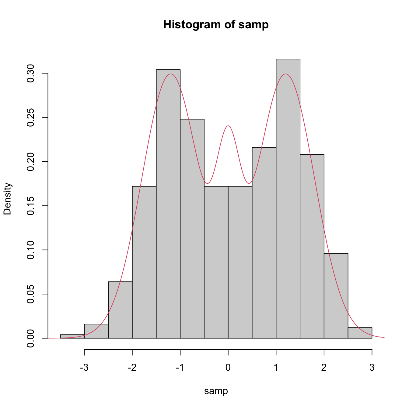


# Plot a MW object directly
# A normal with the same mean and variance is plotted in dashed lines
par(mfrow = c(2, 2))
plot(nor1mix::MW.nm5)
plot(nor1mix::MW.nm7)
plot(nor1mix::MW.nm10)
plot(nor1mix::MW.nm12)
lines(nor1mix::MW.nm1, col = 2:3) # Also possible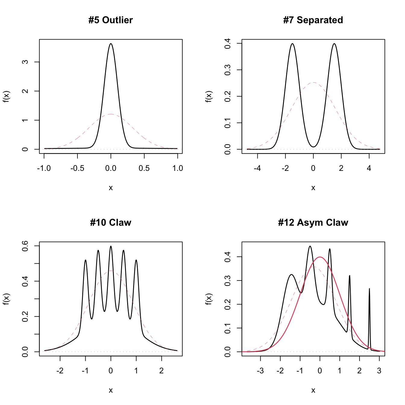

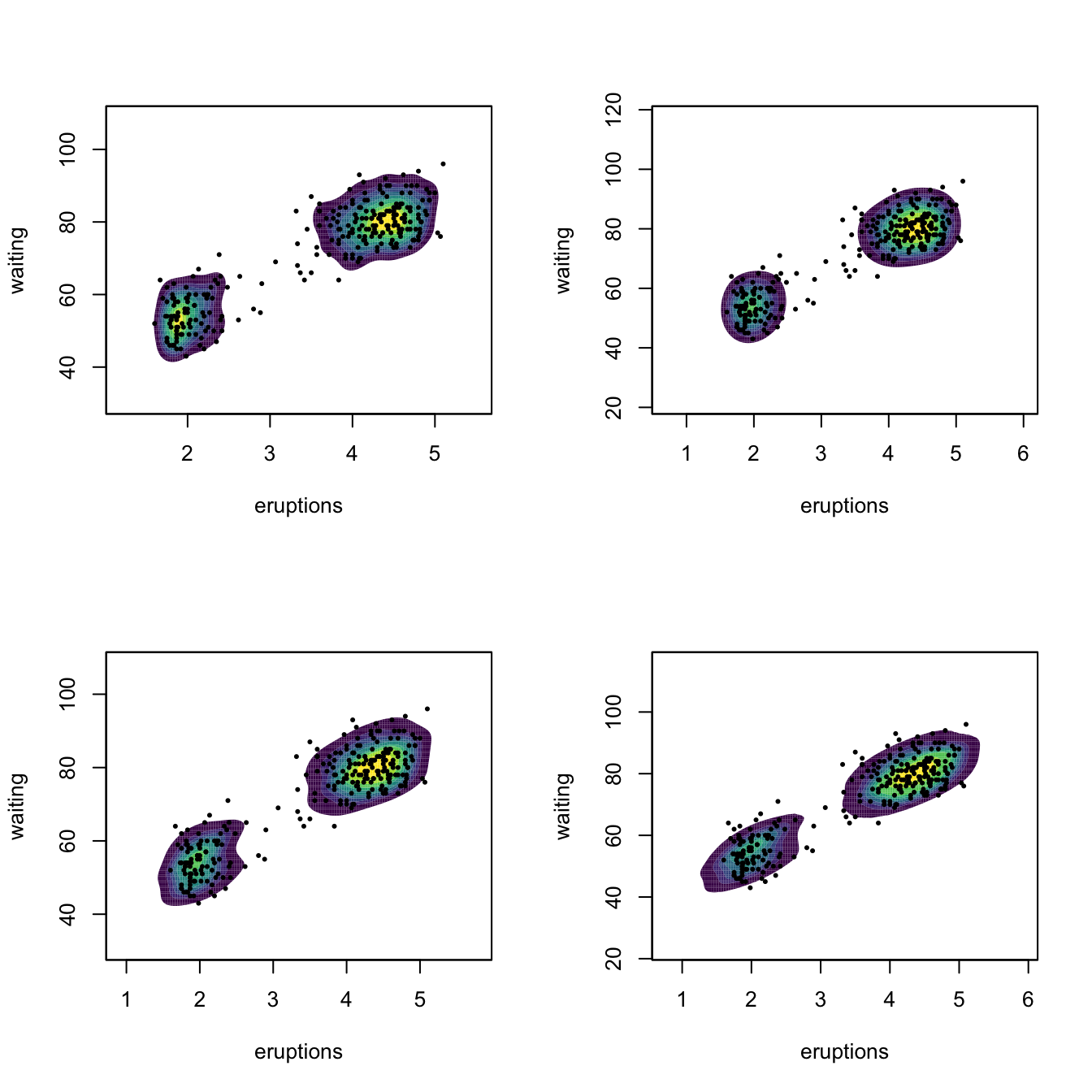
Figure 6.4 presents a visualization of the performance of the kde with different bandwidth selectors, carried out in the family of mixtures of Marron and Wand (1992).

Figure 6.4: Performance comparison of bandwidth selectors. The RT, DPI, LSCV, and BCV are computed for each sample for a normal mixture density. For each sample, computes the ISEs of the selectors and sorts them from best to worst. Changing the scenarios gives insight on the adequacy of each selector to hard- and simple-to-estimate densities. Application also available here.

Which bandwidth selector is the most adequate for a given dataset?

There is no simple and universal answer to this question. There are, however, a series of useful facts and suggestions:

Trying several selectors and inspecting the results may help on determining which one is estimating the density better.
The DPI selector has a convergence rate much faster than the cross-validation selectors. Therefore, in theory, it is expected to perform better than LSCV and BCV. For this reason, it tends to be amongst the preferred bandwidth selectors in the literature.
Cross-validatory selectors may be better suited for highly non-normal and rough densities, in which plug-in selectors may end up oversmoothing.
LSCV tends to be considerably more variable than BCV.
The RT is a quick, simple, and inexpensive selector. However, it tends to give bandwidths that are too large for non-normal data.

6.1.4 Multivariate extension

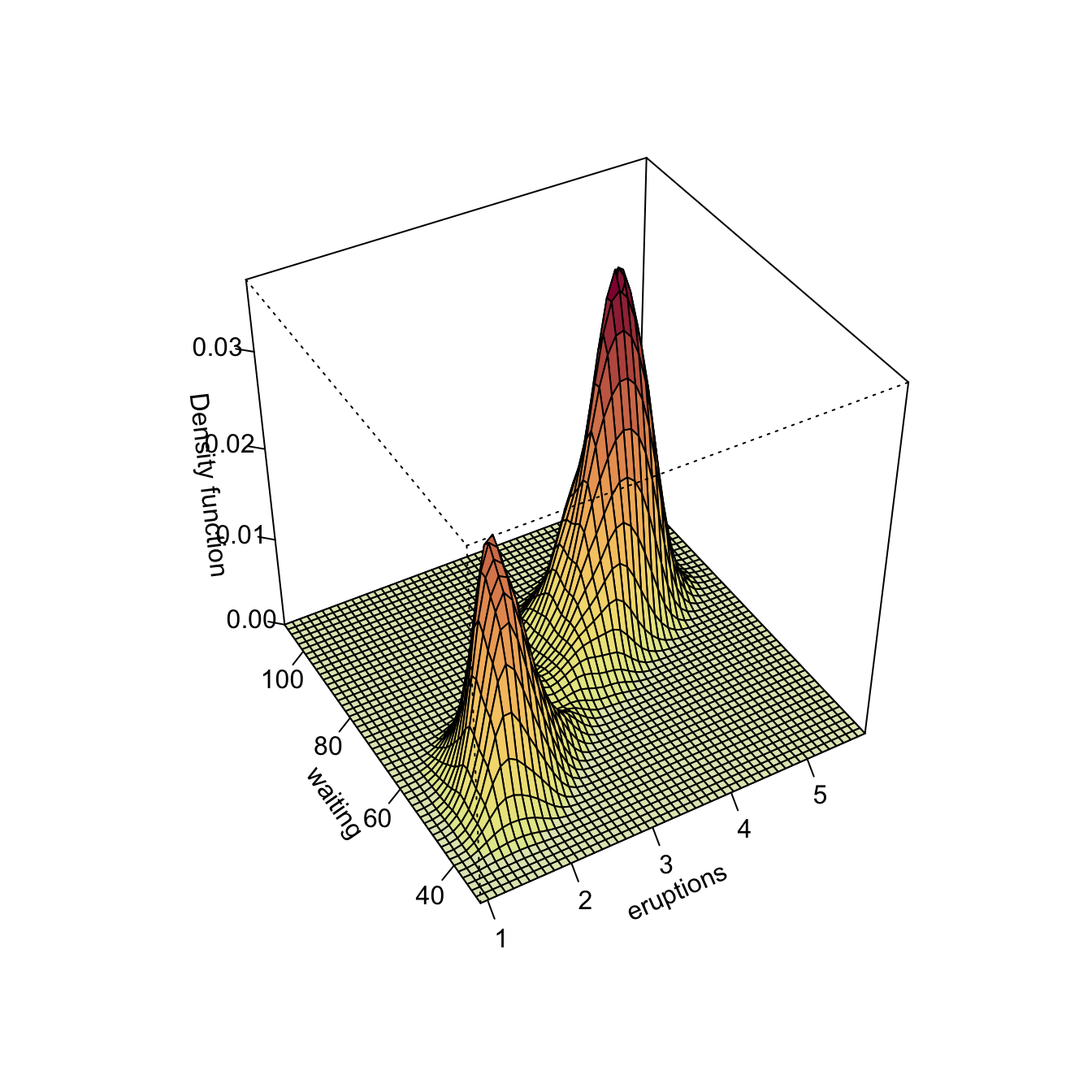
Kernel density estimation can be extended to estimate multivariate densities $f$ in $\mathbb{R}^p.$ For a sample $\mathbf{X}_1,\ldots,\mathbf{X}_n$ in $\mathbb{R}^p,$ the kde of $f$ evaluated at $\mathbf{x}\in\mathbb{R}^p$ is

\[\begin{align} \hat{f}(\mathbf{x};\mathbf{H}):=\frac{1}{n|\mathbf{H}|^{1/2}}\sum_{i=1}^nK\left(\mathbf{H}^{-1/2}(\mathbf{x}-\mathbf{X}_i)\right),\tag{6.9} \end{align}\]

where $K$ is multivariate kernel, a $p$-variate density that is (typically) symmetric and unimodal at $\mathbf{0},$ and that depends on the bandwidth matrix¹⁹⁹ $\mathbf{H},$ a $p\times p$ symmetric and positive definite matrix. A common notation is $K_\mathbf{H}(\mathbf{z}):=|\mathbf{H}|^{-1/2}K\big(\mathbf{H}^{-1/2}\mathbf{z}\big),$ so the kde can be compactly written as $\hat{f}(\mathbf{x};\mathbf{H}):=\frac{1}{n}\sum_{i=1}^nK_\mathbf{H}(\mathbf{x}-\mathbf{X}_i).$ The most employed multivariate kernel is the normal kernel $K(\mathbf{z})=\phi(\mathbf{z};\mathbf{0},\mathbf{I}_p).$

The interpretation of (6.9) is analogous to the one of (6.4): build a mixture of densities with each density centered at each data point. As a consequence, and roughly speaking, most of the concepts and ideas seen in univariate kernel density estimation extend to the multivariate situation, although some of them with considerable technical complications. For example, bandwidth selection inherits the same cross-validatory ideas (LSCV and BCV selectors) and plug-in methods (NS and DPI) seen before, but with increased complexity for the BCV and DPI selectors. The interested reader is referred to Chacón and Duong (2018) for a rigorous and comprehensive treatment.

We briefly discuss next the NS and LSCV selectors, denoted by $\hat{\mathbf{H}}_\mathrm{NS}$ and $\hat{\mathbf{H}}_\mathrm{LSCV},$ respectively. The normal scale bandwidth selector follows, as in the univariate case, by minimizing the asymptotic MISE of the kde, which now takes the form

\[\begin{align*} \mathrm{MISE}[\hat{f}(\cdot;\mathbf{H})]=\mathbb{E}\left[\int (\hat{f}(\mathbf{x};\mathbf{H})-f(\mathbf{x}))^2\,\mathrm{d}\mathbf{x}\right], \end{align*}\]

and then assuming that $f$ is the pdf of a $\mathcal{N}_p\left(\boldsymbol{\mu},\boldsymbol{\Sigma}\right).$ With the normal kernel, this results in

\[\begin{align} \mathbf{H}_\mathrm{NS}=(4(p+2))^{2/(p+4)}n^{-2/(p+4)}\boldsymbol{\Sigma}.\tag{6.10} \end{align}\]

Replacing $\boldsymbol{\Sigma}$ by the sample covariance matrix $\mathbf{S}$ in (6.10) gives $\hat{\mathbf{H}}_\mathrm{NS}.$

The unbiased cross-validation selector neatly extends from the univariate case and attempts to minimize $\mathrm{MISE}[\hat{f}(\cdot;\mathbf{H})]$ by estimating it unbiasedly with

\[\begin{align*} \mathrm{LSCV}(\mathbf{H}):=\int\hat{f}(\mathbf{x};\mathbf{H})^2\,\mathrm{d}\mathbf{x}-2n^{-1}\sum_{i=1}^n\hat{f}_{-i}(\mathbf{X}_i;\mathbf{H}) \end{align*}\]

and then minimizing it:

\[\begin{align} \hat{\mathbf{H}}_\mathrm{LSCV}:=\arg\min_{\mathbf{H}\in\mathrm{SPD}_p}\mathrm{LSCV}(\mathbf{H}),\tag{6.11} \end{align}\]

where $\mathrm{SPD}_p$ is the set of positive definite matrices²⁰⁰ of size $p.$

Considering a full bandwidth matrix $\mathbf{H}$ gives more flexibility to the kde, but also increases notably the amount of bandwidth parameters that need to be chosen – precisely $\frac{p(p+1)}{2}$ – which significantly complicates bandwidth selection as the dimension $p$ grows. A common simplification is to consider a diagonal bandwidth matrix $\mathbf{H}=\mathrm{diag}(h_1^2,\ldots,h_p^2),$ which yields the kde employing product kernels:

\[\begin{align} \hat{f}(\mathbf{x};\mathbf{h})=\frac{1}{n}\sum_{i=1}^nK_{h_1}(x_1-X_{i,1})\times\stackrel{p}{\cdots}\times K_{h_p}(x_p-X_{i,p}),\tag{6.12} \end{align}\]

where $\mathbf{h}=(h_1,\ldots,h_p)'$ is the vector of bandwidths. If the variables $X_1,\ldots,X_p$ have been standardized (so that they have the same scale), then a simple choice is to consider $h=h_1=\ldots=h_p.$

Multivariate kernel density estimation and bandwidth selection is not supported in base R, but the ks package implements the kde by ks::kde for $p\leq6.$ Bandwidth selectors, allowing for full or diagonal bandwidth matrices are implemented by: ks::Hns (NS), ks::Hpi and ks::Hpi.diag (DPI), ks::Hlscv and ks::Hlscv.diag (LSCV), and ks::Hbcv and ks::Hbcv.diag (BCV). The next chunk of code illustrates their usage with the faithful dataset.

# DPI selectors
Hpi1 <- ks::Hpi(x = faithful)
Hpi1
##            [,1]       [,2]
## [1,] 0.06326802  0.6041862
## [2,] 0.60418624 11.1917775

# Compute kde (if H is missing, ks::Hpi is called)
kdeHpi1 <- ks::kde(x = faithful, H = Hpi1)

# Different representations
plot(kdeHpi1, display = "slice", cont = c(25, 50, 75))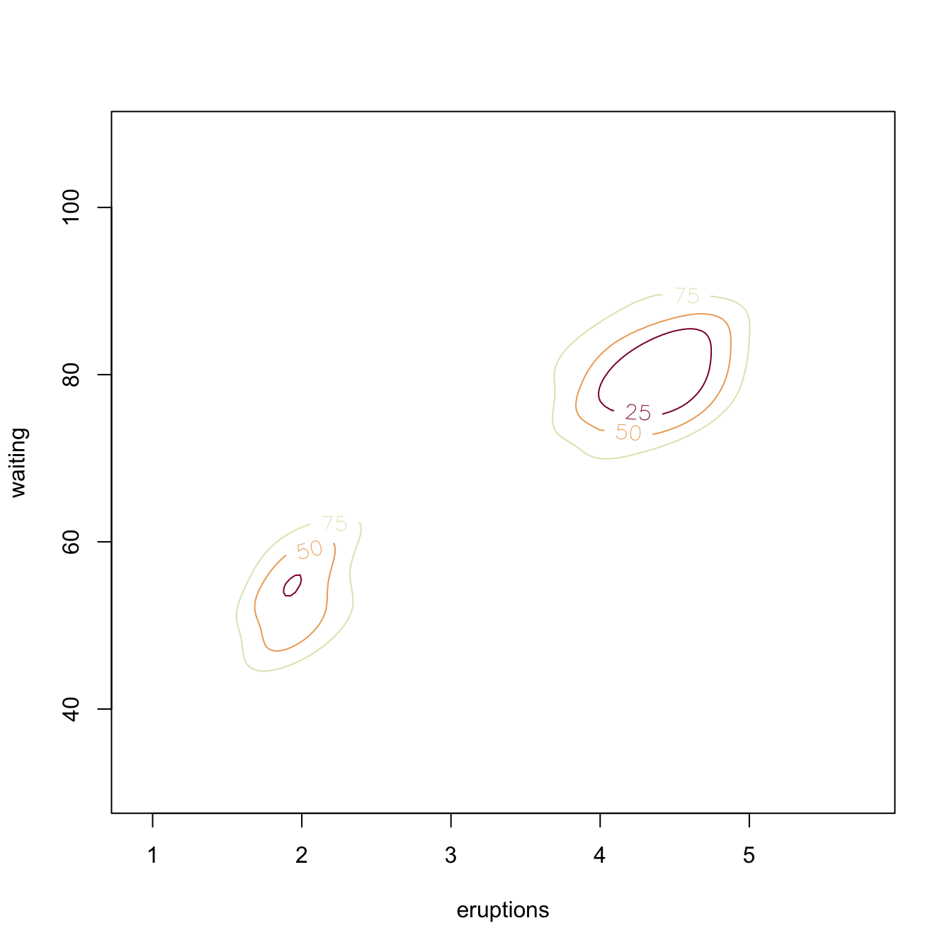

# "cont" specifies the density contours, which are upper percentages of highest
# density regions. The default contours are at 25%, 50%, and 75%
plot(kdeHpi1, display = "filled.contour2", cont = c(25, 50, 75))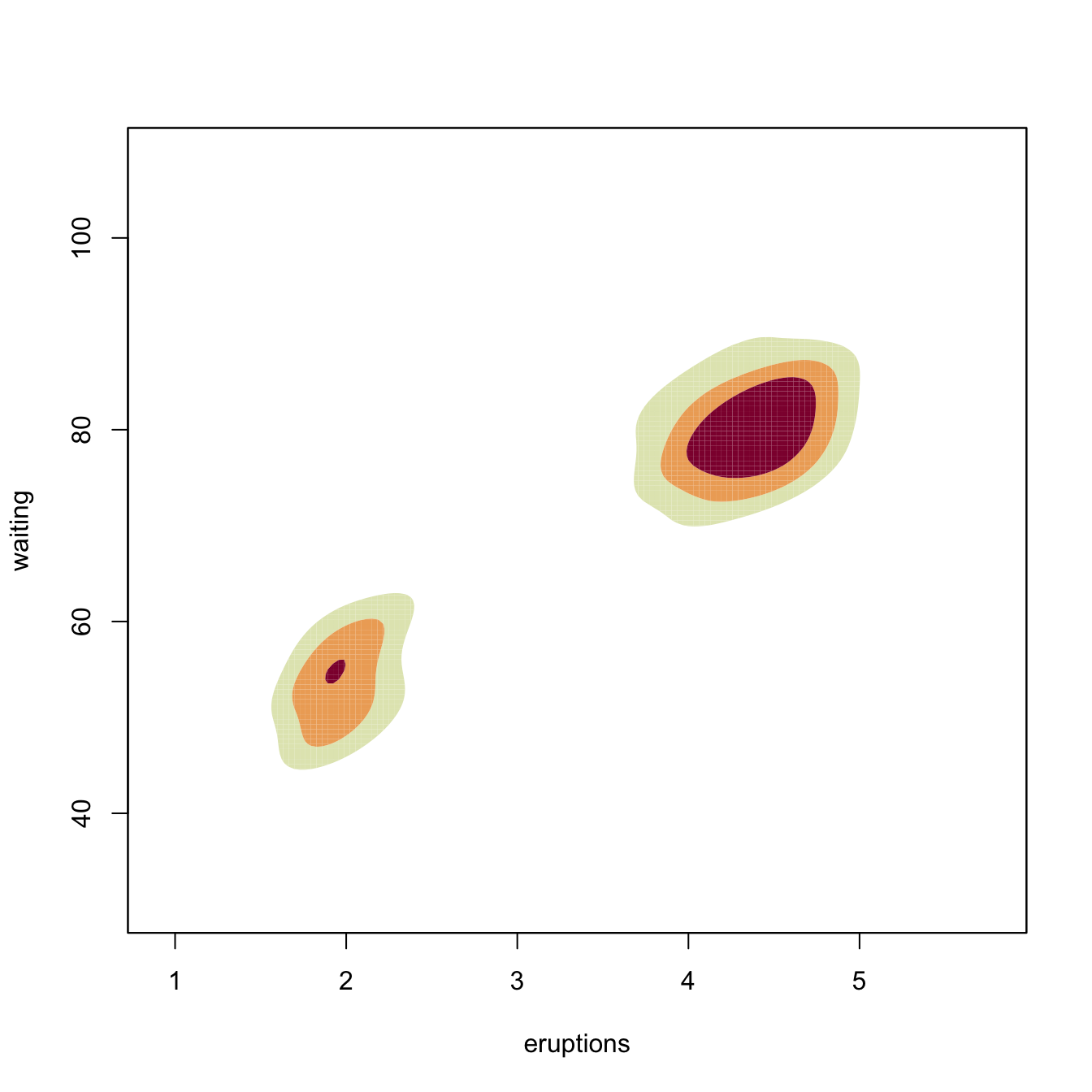

plot(kdeHpi1, display = "persp")


# Manual plotting using the kde object structure
image(kdeHpi1$eval.points[[1]], kdeHpi1$eval.points[[2]],
      kdeHpi1$estimate, col = viridis::viridis(20))
points(kdeHpi1$x)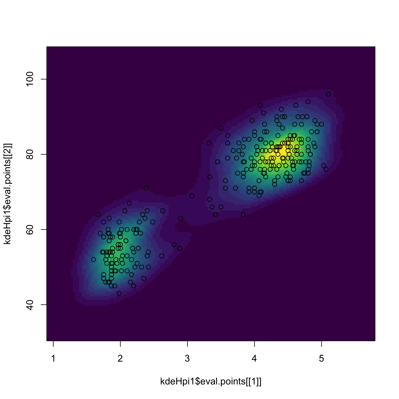


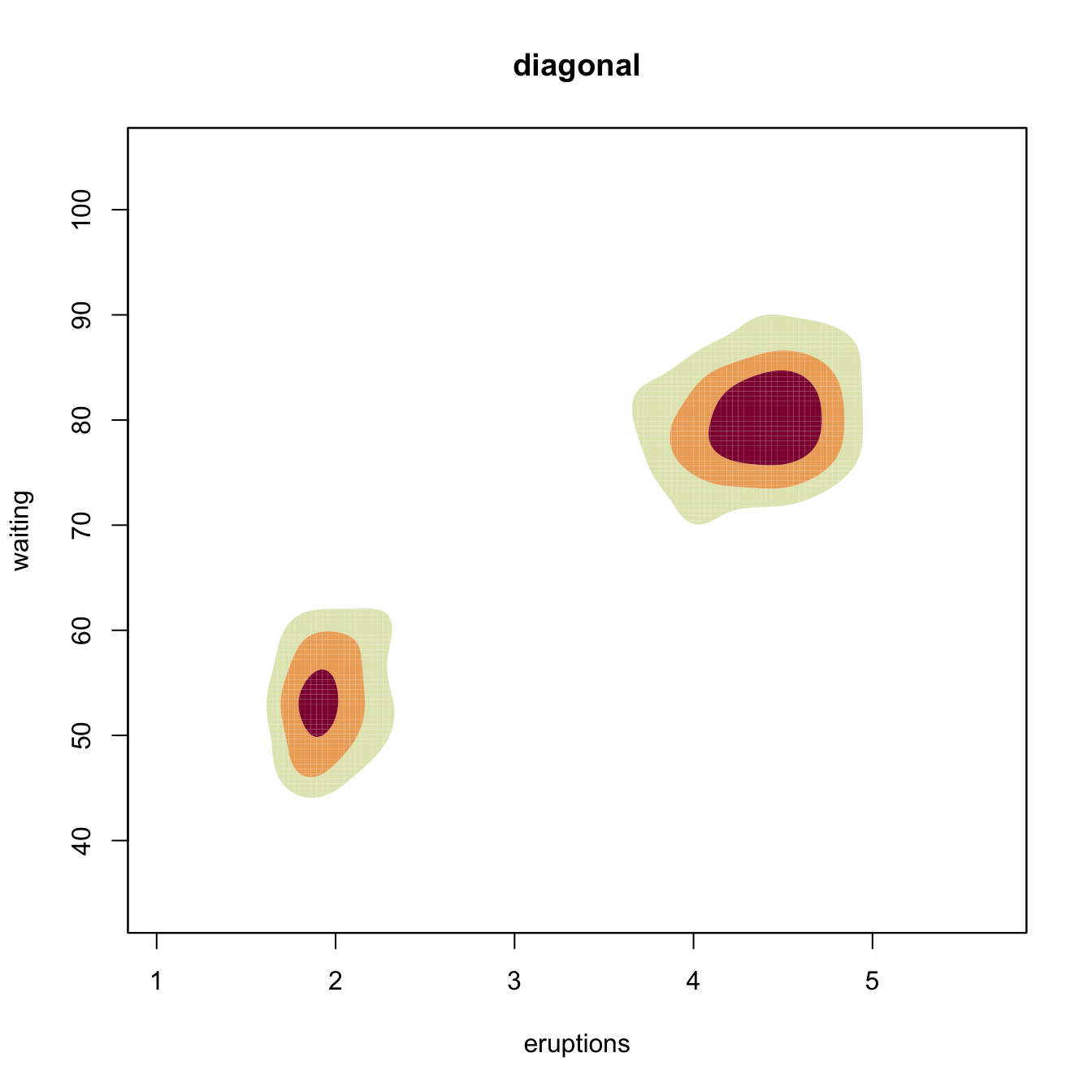
# Diagonal vs. full
Hpi2 <- ks::Hpi.diag(x = faithful)
kdeHpi2 <- ks::kde(x = faithful, H = Hpi2)
plot(kdeHpi1, display = "filled.contour2", cont = c(25, 50, 75),
     main = "full")

plot(kdeHpi2, display = "filled.contour2", cont = c(25, 50, 75),
     main = "diagonal")

# Comparison of selectors along predefined contours
x <- faithful
Hlscv0 <- ks::Hlscv(x = x)
Hbcv0 <- ks::Hbcv(x = x)
Hpi0 <- ks::Hpi(x = x)
Hns0 <- ks::Hns(x = x)
par(mfrow = c(2, 2))
p <- lapply(list(Hlscv0, Hbcv0, Hpi0, Hns0), function(H) {
  # col.fun for custom colors
  plot(ks::kde(x = x, H = H), display = "filled.contour2",
       cont = seq(10, 90, by = 10), col.fun = viridis::viridis)
  points(x, cex = 0.5, pch = 16)
})

Kernel density estimation can be used to visualize density level sets in 3D too, as illustrated as follows with the iris dataset.

# Normal scale bandwidth
Hns1 <- ks::Hns(iris[, 1:3])

# Show high nested contours of high density regions
plot(ks::kde(x = iris[, 1:3], H = Hns1))
rgl::points3d(x = iris[, 1:3])
rgl::rglwidget()

Consider the normal mixture

\[\begin{align*} w_{1}\mathcal{N}_2(\mu_{11},\mu_{12},\sigma_{11}^2,\sigma_{12}^2,\rho_1)+w_{2}\mathcal{N}_2(\mu_{21},\mu_{22},\sigma_{21}^2,\sigma_{22}^2,\rho_2), \end{align*}\]

where $w_1=0.3,$ $w_2=0.7,$ $(\mu_{11}, \mu_{12})=(1, 1),$ $(\mu_{21}, \mu_{22})=(-1, -1),$ $\sigma_{11}^2=\sigma_{21}^2=1,$ $\sigma_{12}^2=\sigma_{22}^2=2,$ $\rho_1=0.5,$ and $\rho_2=-0.5.$

Perform the following simulation exercise:

Plot the density of the mixture using ks::dnorm.mixt and overlay points simulated employing ks::rnorm.mixt. You may want to use ks::contourLevels to have density plots comparable to the kde plots performed in the next step.
Compute the kde employing $\hat{\mathbf{H}}_{\mathrm{DPI}},$ both for full and diagonal bandwidth matrices. Are there any gains on considering full bandwidths? What if $\rho_2=0.7$?
Consider the previous point with $\hat{\mathbf{H}}_{\mathrm{LSCV}}$ instead of $\hat{\mathbf{H}}_{\mathrm{DPI}}.$ Are the conclusions the same?

References

Chacón, J. E., and T. Duong. 2018. Multivariate Kernel Smoothing and Its Applications. Vol. 160. Monographs on Statistics and Applied Probability. Boca Raton: CRC Press. https://doi.org/10.1201/9780429485572.

Marron, J. S., and M. P. Wand. 1992. “Exact Mean Integrated Squared Error.” The Annals of Statistics 20 (2): 712–36. https://doi.org/10.1214/aos/1176348653.

Parzen, E. 1962. “On Estimation of a Probability Density Function and Mode.” Annals of Mathematical Statistics 33 (3): 1065–76. https://doi.org/10.1214/aoms/1177704472.

Rosenblatt, M. 1956. “Remarks on Some Nonparametric Estimates of a Density Function.” Annals of Mathematical Statistics 27 (3): 832–37. https://doi.org/10.1214/aoms/1177728190.

Sheather, S. J., and M. C. Jones. 1991. “A Reliable Data-Based Bandwidth Selection Method for Kernel Density Estimation.” Journal of the Royal Statistical Society, Series B (Methodological) 53 (3): 683–90. https://doi.org/10.1111/j.2517-6161.1991.tb01857.x.

Recall that with this standardization we approach to the probability density concept.↩︎
Note that the function has $2n$ discontinuities that are located at $X_i\pm h.$↩︎
$\mathbb{E}[\mathrm{B}(N,p)]=Np$ and $\mathbb{V}\mathrm{ar}[\mathrm{B}(N,p)]=Np(1-p).$↩︎
Or, in other words, if $h^{-1}$ grows slower than $n.$↩︎
Also known as the Parzen–Rosenblatt estimator to honor the proposals by Parzen (1962) and Rosenblatt (1956).↩︎
Although the efficiency of the normal kernel, with respect to the Epanechnikov kernel, is roughly $0.95.$↩︎
Precisely, the rule-of-thumb given by bw.nrd.↩︎
By solving $\frac{\mathrm{d}}{\mathrm{d} h}\mathrm{AMISE}[\hat{f}(\cdot;h)]=0,$ i.e., $\mu_2^2(K)R(f'')h^3- R(K)n^{-1}h^{-2}=0,$ yields $h_\mathrm{AMISE}.$↩︎
Not to confuse with bw.nrd0!↩︎
The motivation for doing so is to try to add the parametric assumption at a later, less important, step.↩︎
Long intervals containing the solution may lead to unsatisfactory termination of the search; short intervals might not contain the minimum.↩︎
But be careful not expanding the upper limit of the search interval too much!↩︎
Observe that, if $p=1,$ then $\mathbf{H}$ will equal the square of the bandwidth $h,$ that is, $\mathbf{H}=h^2.$↩︎
Observe that implementing the optimization of (6.11) is not trivial, since it is required to enforce the constraint $\mathbf{H}\in\mathrm{SPD}_p.$ A neat way of parametrizing $\mathbf{H}$ that induces the positive definiteness constrain is through the (unique) Cholesky decomposition of $\mathbf{H}\in\mathrm{SPD}_p$: $\mathbf{H}=\mathbf{R}'\mathbf{R},$ where $\mathbf{R}$ is a triangular matrix with positive entries on the diagonal (but the remaining entries unconstrained). Therefore, optimization of (6.11) can be done through the $\frac{p(p+1)}{2}$ entries of $\mathbf{R}.$↩︎