A.1 Informal review on hypothesis testing

The process of hypothesis testing has an interesting analogy with a (simplified) trial. The analogy helps understanding the elements present in a formal hypothesis test in an intuitive way.

Hypothesis test	Trial
Null hypothesis $H_0$	The defendant: an individual accused of committing a crime. He is backed up by the presumption of innocence, which means that he is not guilty until there are enough evidences to support his guilt.
Sample $X_1,\ldots,X_n$	Collection of small evidences supporting innocence and guilt of the defendant. These evidences contain a certain degree of uncontrollable randomness due to how they were collected and the context regarding the case²³⁴.
Test statistic²³⁵ $T_n$	Summary of the evidences presented by the prosecutor and defense lawyer.
Distribution of $T_n$ under $H_0$	The judge conducting the trial. Evaluates and measures the evidence presented by both sides and presents a verdict for the defendant.
Significance level $\alpha$	$1-\alpha$ is the strength of evidences required by the judge for condemning the defendant. The judge allows evidences that, on average, condemn $100\alpha\%$ of the innocents, due to the randomness inherent to the evidences collection process. The level $\alpha=0.05$ is considered to be reasonable²³⁶.
$p$-value	Decision of the judge that measures the degree of compatibility, in a scale $0$–$1,$ of the presumption of innocence with the summary of the evidences presented. If $p\text{-value}<\alpha,$ the defendant is declared guilty, as the evidences supporting its guilt are strong enough to override his presumption of innocence. Otherwise, he is declared not guilty.
$H_0$ is rejected	The defendant is declared guilty: there are strong evidences supporting its guilt.
$H_0$ is not rejected	The defendant is declared not guilty: either he is innocent or there are not enough evidences supporting his guilt.

More formally, the $p$-value of an hypothesis test about $H_0$ is defined as:

The $p$-value is the probability of obtaining a test statistic more unfavourable to $H_0$ than the observed, assuming that $H_0$ is true.

Therefore, if the $p$-value is small (smaller than the chosen level $\alpha$), it is unlikely that the evidences against $H_0$ are due to randomness. As a consequence, $H_0$ is rejected. If the $p$-value is large (larger than $\alpha$), then it is more likely that the evidences against $H_0$ are merely due to the randomness of the data. In this case, we do not reject $H_0.$

If $H_0$ holds, then the $p$-value (which is a random variable) is distributed uniformly in $(0,1).$ If $H_0$ does not hold, then the distribution of the $p$-value is not uniform but concentrated at $0$ (where the rejections of $H_0$ take place).

Let’s quickly illustrate the previous fact with the well-known Kolmogorov–Smirnov test. This test evaluates whether the unknown cdf of $X,$ $F,$ equals a specified cdf $F_0.$ In other words, it tests the null hypothesis²³⁷

\[\begin{align*} H_0:F=F_0 \end{align*}\]

versus the alternative hypothesis²³⁸

\[\begin{align*} H_1:F\neq F_0. \end{align*}\]

For that purpose, given a sample $X_1,\ldots,X_n$ of $X,$ the Kolmogorov–Smirnov statistic $D_n$ is computed:

\[\begin{align} D_n:=&\,\sqrt{n}\sup_{x\in\mathbb{R}} \left|F_n(x)-F_0(x)\right|=\max(D_n^+,D_n^-),\tag{A.1}\\ D_n^+:=&\,\sqrt{n}\max_{1\leq i\leq n}\left\{\frac{i}{n}-U_{(i)}\right\},\nonumber\\ D_n^-:=&\,\sqrt{n}\max_{1\leq i\leq n}\left\{U_{(i)}-\frac{i-1}{n}\right\}.\nonumber \end{align}\]

where $F_n$ represents the empirical cdf of $X_1,\ldots,X_n$ and $U_{(j)}$ stands for the $j$-th sorted $U_i:=F_0(X_i),$ $i=1,\ldots,n.$ If $H_0$ holds, then $D_n$ tends to be small. Conversely, when $F\neq F_0,$ larger values of $D_n$ are expected, so the test rejects when $D_n$ is large.

If $H_0$ holds, then $D_n$ has an asymptotic²³⁹ cdf given by the Kolmogorov–Smirnov’s $K$ function:

\[\begin{align} \lim_{n\to\infty}\mathbb{P}[D_n\leq x]=K(x):=1-2\sum_{m=1}^\infty (-1)^{m-1}e^{-2m^2x^2}.\tag{A.2} \end{align}\]

The test statistic $D_n,$ the asymptotic cdf $K,$ and the associated asymptotic $p$-value²⁴⁰ are readily implemented in R through the ks.test function.

Implement the Kolmogorov–Smirnov test from the equations above. This amounts to:

Provide a function for computing the test statistic (A.1) from a sample $X_1,\ldots,X_n$ and a cdf $F_0.$
Implement the $K$ function (A.2).
Call the previous functions from a routine that returns the asymptotic $p$-value of the test.

Compare that the implementations coincide with the ones of the ks.test function when exact = FALSE. Note: ks.test computes $D_n/\sqrt{n}$ instead of $D_n.$

# Sample data from a N(0, 1)
set.seed(3245678)
n <- 50
x <- rnorm(n)

# Kolmogorov-Smirnov test for H_0 : F = N(0, 1). Does not reject.
ks.test(x, "pnorm")
## 
##  Exact one-sample Kolmogorov-Smirnov test
## 
## data:  x
## D = 0.050298, p-value = 0.9989
## alternative hypothesis: two-sided

# Simulation of p-values when H_0 is true
M <- 1e4
pValues_H0 <- sapply(1:M, function(i) {
  x <- rnorm(n) # N(0, 1)
  ks.test(x, "pnorm")$p.value
})

# Simulation of p-values when H_0 is false -- the data does not
# come from a N(0, 1) but from a N(0, 1.5)
pValues_H1 <- sapply(1:M, function(i) {
  x <- rnorm(n, mean = 0, sd = sqrt(1.5)) # N(0, 1.5)
  ks.test(x, "pnorm")$p.value
})

# Comparison of p-values
par(mfrow = 1:2)
hist(pValues_H0, breaks = seq(0, 1, l = 20), probability = TRUE,
     main = expression(H[0]), ylim = c(0, 2.5))
abline(h = 1, col = 2)
hist(pValues_H1, breaks = seq(0, 1, l = 20), probability = TRUE,
     main = expression(H[1]), ylim = c(0, 2.5))
abline(h = 1, col = 2)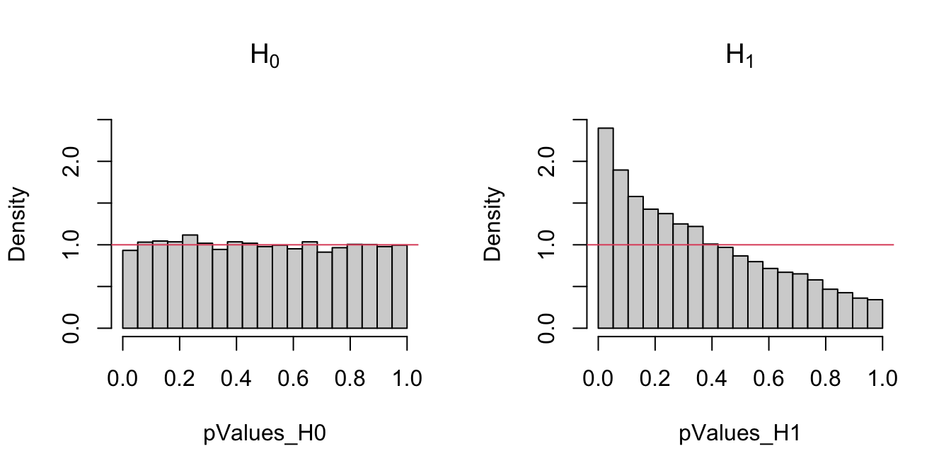

$Comparison of the distribution of $p$-values under $H_0$ and $H_1$ for the Kolmogorov–Smirnov test. Observe that the frequency of low $p$-values, associated with the rejection of $H_0,$ grows when $H_0$ does not hold. Under $H_0,$ the distribution of the $p$-values is uniform.$

Figure A.1: Comparison of the distribution of $p$-values under $H_0$ and $H_1$ for the Kolmogorov–Smirnov test. Observe that the frequency of low $p$-values, associated with the rejection of $H_0,$ grows when $H_0$ does not hold. Under $H_0,$ the distribution of the $p$-values is uniform.

Think about phenomena that may randomly support innoncence or guilt of the defendant, irrespective of his true condition. For example: spurious coincidences (“happen to be in the wrong place at the wrong time”), lost of evidences during the case, previous past statemets of the defendant, doubtious identification by witness, imprecise witness testimonies, unverificable alibi, etc.↩︎
Usually simply referred to as statistic.↩︎
As the judge has to have the power of condemning a guilty defendant. Setting $\alpha=0$ (no innocents are declared guilt) would result in a judge that systematically declares everybody not guilty. Therefore, a compromise is needed.↩︎
Understood as $F(x)=F_0(x)$ for $x\in\mathbb{R}.$ For $F\neq F_0,$ we mean that $F(x)\neq F_0(x)$ for at least one $x\in\mathbb{R}.$↩︎
Formally, a null hypothesis $H_0$ is tested against an alternative hypothesis $H_1.$ The concept of alternative hypothesis was not addressed in the trial analogy for the sake of simplicity, but you may think of $H_1$ as the defendant being not guilty or as the plaintiff or complainant. The alternative hypothesis $H_1$ represents the “alternative truth” to $H_0$ and the test decides between $H_0$ and $H_1,$ only rejecting $H_0$ in favor of $H_1$ if there are enough evidences on the data against $H_0$ or supporting $H_1.$ Obviously, $H_0\cap H_1=\emptyset.$ But recall that also $H_1\subset \neg H_0$ or, in other words, $H_1$ may be more restrictive than the negation of $H_0.$↩︎
When the sample size $n$ is large: $n\to\infty.$↩︎
Which is $\lim_{n\to\infty}\mathbb{P}[d_n>D_n]=1-K(d_n),$ where $d_n$ is the observed statistic and $D_n$ is the random variable (A.1).↩︎

Hypothesis test	Trial
Null hypothesis \(H_0\)	The defendant: an individual accused of committing a crime. He is backed up by the presumption of innocence, which means that he is not guilty until there are enough evidences to support his guilt.
Sample \(X_1,\ldots,X_n\)	Collection of small evidences supporting innocence and guilt of the defendant. These evidences contain a certain degree of uncontrollable randomness due to how they were collected and the context regarding the case²³⁴.
Test statistic²³⁵ \(T_n\)	Summary of the evidences presented by the prosecutor and defense lawyer.
Distribution of \(T_n\) under \(H_0\)	The judge conducting the trial. Evaluates and measures the evidence presented by both sides and presents a verdict for the defendant.
Significance level \(\alpha\)	\(1-\alpha\) is the strength of evidences required by the judge for condemning the defendant. The judge allows evidences that, on average, condemn \(100\alpha\%\) of the innocents, due to the randomness inherent to the evidences collection process. The level \(\alpha=0.05\) is considered to be reasonable²³⁶.
\(p\)-value	Decision of the judge that measures the degree of compatibility, in a scale \(0\)–\(1,\) of the presumption of innocence with the summary of the evidences presented. If \(p\text{-value}<\alpha,\) the defendant is declared guilty, as the evidences supporting its guilt are strong enough to override his presumption of innocence. Otherwise, he is declared not guilty.
\(H_0\) is rejected	The defendant is declared guilty: there are strong evidences supporting its guilt.
\(H_0\) is not rejected	The defendant is declared not guilty: either he is innocent or there are not enough evidences supporting his guilt.