6.5 Local likelihood
We explore in this section an extension of the local polynomial estimator that reproduces the extension generalized linear models made of linear models. This extension aims to estimate the regression function by relying in the likelihood, rather than the least squares. Thus, the idea behind the local likelihood is to fit, locally, parametric models by maximum likelihood.
We begin by seeing that local likelihood using the linear model is equivalent to local polynomial modeling. Theorem A.1 shows that, under the assumptions given in Section 2.3, the ML estimate of \(\boldsymbol{\beta}\) in the linear model
\[\begin{align} Y|(X_1,\ldots,X_p)\sim\mathcal{N}(\beta_0+\beta_1X_1+\cdots+\beta_pX_p,\sigma^2)\tag{6.29} \end{align}\]
is equivalent to the least squares estimate, \(\hat{\boldsymbol{\beta}}=(\mathbf{X}'\mathbf{X})^{-1}\mathbf{X}'\mathbf{Y}.\) The reason was the form of the conditional (on \(X_1,\ldots,X_p\)) likelihood:
\[\begin{align*} \ell(\boldsymbol{\beta})=&\,-\frac{n}{2}\log(2\pi\sigma^2)\nonumber\\ &-\frac{1}{2\sigma^2}\sum_{i=1}^n(Y_i-\beta_0-\beta_1X_{i1}-\cdots-\beta_pX_{ip})^2. \end{align*}\]
If there is a single predictor \(X,\) polynomial fitting of order \(p\) of the conditional mean can be achieved by the well-known trick of identifying the \(j\)-th predictor \(X_j\) in (6.29) by \(X^j.\) This results in
\[\begin{align} Y|X\sim\mathcal{N}(\beta_0+\beta_1X+\cdots+\beta_pX^p,\sigma^2).\tag{6.30} \end{align}\]
Therefore, the weighted log-likelihood of the linear model (6.30) about \(x\) is
\[\begin{align} \ell_{x,h}(\boldsymbol{\beta})=&\,-\frac{n}{2}\log(2\pi\sigma^2)\nonumber\\ &-\frac{1}{2\sigma^2}\sum_{i=1}^n(Y_i-\beta_0-\beta_1X_i-\cdots-\beta_pX_i^p)^2K_h(x-X_i).\tag{6.31} \end{align}\]
Maximizing with respect to \(\boldsymbol{\beta}\) the local log-likelihood (6.31) provides \(\hat\beta_0=\hat{m}(x;p,h),\) the local polynomial estimator, as it was obtained in (6.21), but now from a likelihood-based perspective. The key insight is to realize that the very same idea can be applied to the family of generalized linear models.
Figure 6.7: Construction of the local likelihood estimator. The animation shows how local likelihood fits in a neighborhood of \(x\) are combined to provide an estimate of the regression function for binary response, which depends on the polynomial degree, bandwidth, and kernel (gray density at the bottom). The data points are shaded according to their weights for the local fit at \(x.\) Application available here.
We illustrate the local likelihood principle for the logistic regression. In this case, \(\{(x_i,Y_i)\}_{i=1}^n\) with
\[\begin{align*} Y_i|X_i=x_i\sim \mathrm{Ber}(\mathrm{logistic}(\eta(x_i))),\quad i=1,\ldots,n, \end{align*}\]
with the polynomial term234
\[\begin{align*} \eta(x):=\beta_0+\beta_1x+\cdots+\beta_px^p. \end{align*}\]
The log-likelihood of \(\boldsymbol{\beta}\) is
\[\begin{align*} \ell(\boldsymbol{\beta}) =&\,\sum_{i=1}^n\left\{Y_i\log(\mathrm{logistic}(\eta(x_i)))+(1-Y_i)\log(1-\mathrm{logistic}(\eta(x_i)))\right\}\nonumber\\ =&\,\sum_{i=1}^n\ell(Y_i,\eta(x_i)), \end{align*}\]
where we consider the log-likelihood addend \(\ell(y,\eta)=y\eta-\log(1+e^\eta),\) and make explicit the dependence on \(\eta(x)\) for clarity in the next developments (and implicit the dependence on \(\boldsymbol{\beta}\)).
The local log-likelihood of \(\boldsymbol{\beta}\) about \(x\) is then
\[\begin{align} \ell_{x,h}(\boldsymbol{\beta}) :=\sum_{i=1}^n\ell(Y_i,\eta(X_i-x))K_h(x-X_i).\tag{6.32} \end{align}\]
Maximizing235 the local log-likelihood (6.32) with respect to \(\boldsymbol{\beta}\) provides
\[\begin{align*} \hat{\boldsymbol{\beta}}_{h}=\arg\max_{\boldsymbol{\beta}\in\mathbb{R}^{p+1}}\ell_{x,h}(\boldsymbol{\beta}), \end{align*}\]
where \(\hat{\boldsymbol{\beta}}_{h}=(\hat{\beta}_{h,0},\hat{\beta}_{h,1},\ldots,\hat{\beta}_{h,p})'.\) The local likelihood estimate of \(\eta(x)\) is
\[\begin{align*} \hat\eta(x):=\hat\beta_{h,0}. \end{align*}\]
Note that the dependence of \(\hat\beta_0\) on \(x\) and \(h\) is omitted. From \(\hat\eta(x),\) we can obtain the local logistic regression evaluated at \(x\) as
\[\begin{align} \hat{m}_{\ell}(x;h,p):=g^{-1}\left(\hat\eta(x)\right)=\mathrm{logistic}(\hat\beta_{h,0}).\tag{6.33} \end{align}\]
Each evaluation of \(\hat{m}_{\ell}(x;h,p)\) in a different \(x\) requires, thus, a weighted fit of the underlying logistic model.
The code below shows three different ways of implementing the local logistic regression (of first degree) in R.
# Simulate some data
n <- 200
logistic <- function(x) 1 / (1 + exp(-x))
p <- function(x) logistic(1 - 3 * sin(x))
set.seed(123456)
X <- runif(n = n, -3, 3)
Y <- rbinom(n = n, size = 1, prob = p(X))

# Set bandwidth and evaluation grid
h <- 0.25
x <- seq(-3, 3, l = 501)

# Approach 1: optimize the weighted log-likelihood through the workhorse
# function underneath glm, glm.fit
suppressWarnings(
  fitGlm <- sapply(x, function(x) {
    K <- dnorm(x = x, mean = X, sd = h)
    glm.fit(x = cbind(1, X - x), y = Y, weights = K,
            family = binomial())$coefficients[1]
  })
)

# Approach 2: optimize directly the weighted log-likelihood
suppressWarnings(
  fitNlm <- sapply(x, function(x) {
    K <- dnorm(x = x, mean = X, sd = h)
    nlm(f = function(beta) {
      -sum(K * (Y * (beta[1] + beta[2] * (X - x)) -
                  log(1 + exp(beta[1] + beta[2] * (X - x)))))
      }, p = c(0, 0))$estimate[1]
  })
)

# Approach 3: employ locfit::locfit
# Bandwidth cannot be controlled explicitly -- only through nn in ?lp
fitLocfit <- locfit::locfit(Y ~ locfit::lp(X, deg = 1, nn = h),
                            family = "binomial", kern = "gauss")

# Compare fits
plot(x, p(x), ylim = c(0, 1.5), type = "l", lwd = 2)
lines(x, logistic(fitGlm), col = 2)
lines(x, logistic(fitNlm), col = 3, lty = 2)
plot(fitLocfit, add = TRUE, col = 4)
legend("topright", legend = c("p(x)", "glm", "nlm", "locfit"), lwd = 2,
       col = c(1, 2, 3, 4), lty = c(1, 1, 2, 1))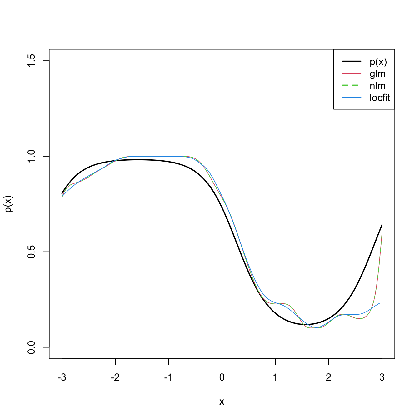
Bandwidth selection can be done by means of likelihood cross-validation. The objective is to maximize the local likelihood fit at \((x_i,Y_i)\) but removing the influence by the datum itself. That is, maximizing
\[\begin{align} \mathrm{LCV}(h)=\sum_{i=1}^n\ell(Y_i,\hat\eta_{-i}(X_i)),\tag{6.34} \end{align}\]
where \(\hat\eta_{-i}(x_i)\) represents the local fit at \(x_i\) without the \(i\)-th datum \((x_i,Y_i).\) Unfortunately, the nonlinearity of (6.33) forbids a simplifying result as Proposition 6.1. Thus, in principle,236 it is required to fit \(n\) local likelihoods for sample size \(n-1\) for obtaining a single evaluation of (6.34).
We conclude by illustrating how to compute the LCV function and optimize it (keep in mind that much more efficient implementations are possible!).
# Exact LCV -- recall that we *maximize* the LCV!
h <- seq(0.1, 2, by = 0.1)
suppressWarnings(
  LCV <- sapply(h, function(h) {
  sum(sapply(1:n, function(i) {
    K <- dnorm(x = X[i], mean = X[-i], sd = h)
    nlm(f = function(beta) {
      -sum(K * (Y[-i] * (beta[1] + beta[2] * (X[-i] - X[i])) -
                  log(1 + exp(beta[1] + beta[2] * (X[-i] - X[i])))))
      }, p = c(0, 0))$minimum
    }))
  })
)
plot(h, LCV, type = "o")
abline(v = h[which.max(LCV)], col = 2)
References
If \(p=1,\) then we have the usual simple logistic model.↩︎
No analytical solution for the optimization problem, numerical optimization is needed.↩︎
The interested reader is referred to Sections 4.3.3 and 4.4.3 of Loader (1999) for an approximation of (6.34) that only requires a local likelihood fit for a single sample.↩︎