1.3 General notation and background

We use capital letters to denote random variables, such as $X,$ and lowercase, such as $x,$ to denote deterministic values. For example $\mathbb{P}[X=x]$ means “the probability that the random variable $X$ takes the particular value $x$ ”. In predictive modeling we are concerned about the prediction or explanation of a response $Y$ from a set of predictors $X_1,\ldots,X_p.$ Both $Y$ and $X_1,\ldots,X_p$ are random variables, but we use them in a different way: our interest lies in predicting or explaining $Y$ from $X_1,\ldots,X_p.$ Other name for $Y$ is dependent variable and $X_1,\ldots,X_p$ are sometimes referred to as independent variables, covariates, or explanatory variables. We will not use these terminologies.

The cumulative distribution function (cdf) of a random variable $X$ is $F(x):=\mathbb{P}[X\leq x]$ and is a function that completely characterizes the randomness of $X.$ Continuous random variables are also characterized by the probability density function (pdf) $f(x)=F'(x),$ ⁹ which represents the infinitesimal relative probability of $X$ per unit of length. On the other hand, discrete random variables are also characterized by the probability mass function $\mathbb{P}[X= x].$ We write $X\sim F$ (or $X\sim f$ if $X$ is continuous) to denote that $X$ has a cdf $F$ (or a pdf $f$ ). If two random variables $X$ and $Y$ have the same distribution, we write $X\stackrel{d}{=}Y.$

For a random variable $X\sim F,$ the expectation of $g(X)$ is defined as¹⁰

$\begin{align*} \mathbb{E}[g(X)]:=&\,\int g(x)\,\mathrm{d}F(x)\\ :=&\, \begin{cases} \displaystyle\int g(x)f(x)\,\mathrm{d}x,&\text{ if }X\text{ is continuous,}\\\displaystyle\sum_{\{x\in\mathbb{R}:\mathbb{P}[X=x]>0\}} g(x)\mathbb{P}[X=x],&\text{ if }X\text{ is discrete.} \end{cases} \end{align*}$

The sign “ $:=$ ” emphasizes that the Left Hand Side (LHS) of the equality is defined for the first time as the Right Hand Side (RHS). Unless otherwise stated, the integration limits of any integral are $\mathbb{R}$ or $\mathbb{R}^p.$ The variance is defined as $\mathbb{V}\mathrm{ar}[X]:=\mathbb{E}[(X-\mathbb{E}[X])^2]=\mathbb{E}[X^2]-\mathbb{E}[X]^2.$

We employ boldface to denote vectors (assumed to be column matrices, although sometimes written in row-layout), like $\mathbf{a},$ and matrices, like $\mathbf{A}.$ We denote by $\mathbf{A}'$ to the transpose of $\mathbf{A}.$ Boldfaced capitals will be used simultaneously for denoting matrices and also random vectors $\mathbf{X}=(X_1,\ldots,X_p),$ which are collections of random variables $X_1,\ldots,X_p.$ The (joint) cdf of $\mathbf{X}$ is¹¹

$\begin{align*} F(\mathbf{x}):=\mathbb{P}[\mathbf{X}\leq \mathbf{x}]:=\mathbb{P}[X_1\leq x_1,\ldots,X_p\leq x_p] \end{align*}$

and, if $\mathbf{X}$ is continuous, its (joint) pdf is $f:=\frac{\partial^p}{\partial x_1\cdots\partial x_p}F.$

The marginals of $F$ and $f$ are the cdf and pdf of $X_j,$ $j=1,\ldots,p,$ respectively. They are defined as:

$\begin{align*} F_{X_j}(x_j)&:=\mathbb{P}[X_j\leq x_j]=F(\infty,\ldots,\infty,x_j,\infty,\ldots,\infty),\\ f_{X_j}(x_j)&:=\frac{\partial}{\partial x_j}F_{X_j}(x_j)=\int_{\mathbb{R}^{p-1}} f(\mathbf{x})\,\mathrm{d}\mathbf{x}_{-j}, \end{align*}$

where $\mathbf{x}_{-j}:=(x_1,\ldots,x_{j-1},x_{j+1},\ldots,x_p).$ The definitions can be extended analogously to the marginals of the cdf and pdf of different subsets of $\mathbf{X}.$

The conditional cdf and pdf of $X_1|(X_2,\ldots,X_p)$ are defined, respectively, as

$\begin{align*} F_{X_1| \mathbf{X}_{-1}=\mathbf{x}_{-1}}(x_1)&:=\mathbb{P}[X_1\leq x_1| \mathbf{X}_{-1}=\mathbf{x}_{-1}],\\ f_{X_1| \mathbf{X}_{-1}=\mathbf{x}_{-1}}(x_1)&:=\frac{f(\mathbf{x})}{f_{\mathbf{X}_{-1}}(\mathbf{x}_{-1})}. \end{align*}$

The conditional expectation of $Y| X$ is the following random variable¹²

$\begin{align*} \mathbb{E}[Y| X]:=\int y \,\mathrm{d}F_{Y| X}(y| X). \end{align*}$

For two random variables $X_1$ and $X_2,$ the covariance between them is defined as

$\begin{align*} \mathrm{Cov}[X_1,X_2]:=\mathbb{E}[(X_1-\mathbb{E}[X_1])(X_2-\mathbb{E}[X_2])]=\mathbb{E}[X_1X_2]-\mathbb{E}[X_1]\mathbb{E}[X_2], \end{align*}$

and the correlation between them is defined as

$\begin{align*} \mathrm{Cor}[X_1,X_2]:=\frac{\mathrm{Cov}[X_1,X_2]}{\sqrt{\mathbb{V}\mathrm{ar}[X_1]\mathbb{V}\mathrm{ar}[X_2]}}. \end{align*}$

The variance and the covariance are extended to a random vector $\mathbf{X}=(X_1,\ldots,X_p)'$ by means of the so-called variance-covariance matrix:

$\begin{align*} \mathbb{V}\mathrm{ar}[\mathbf{X}]:=&\,\mathbb{E}[(\mathbf{X}-\mathbb{E}[\mathbf{X}])(\mathbf{X}-\mathbb{E}[\mathbf{X}])']\\ =&\,\mathbb{E}[\mathbf{X}\mathbf{X}']-\mathbb{E}[\mathbf{X}]\mathbb{E}[\mathbf{X}]'\\ =&\,\begin{pmatrix} \mathbb{V}\mathrm{ar}[X_1] & \mathrm{Cov}[X_1,X_2] & \cdots & \mathrm{Cov}[X_1,X_p]\\ \mathrm{Cov}[X_2,X_1] & \mathbb{V}\mathrm{ar}[X_2] & \cdots & \mathrm{Cov}[X_2,X_p]\\ \vdots & \vdots & \ddots & \vdots \\ \mathrm{Cov}[X_p,X_1] & \mathrm{Cov}[X_p,X_2] & \cdots & \mathbb{V}\mathrm{ar}[X_p]\\ \end{pmatrix}, \end{align*}$

where $\mathbb{E}[\mathbf{X}]:=(\mathbb{E}[X_1],\ldots,\mathbb{E}[X_p])'$ is just the componentwise expectation. As in the univariate case, the expectation is a linear operator, which now means that

$\begin{align} \mathbb{E}[\mathbf{A}\mathbf{X}+\mathbf{b}]=\mathbf{A}\mathbb{E}[\mathbf{X}]+\mathbf{b},\quad\text{for a $q\times p$ matrix } \mathbf{A}\text{ and }\mathbf{b}\in\mathbb{R}^q.\tag{1.2} \end{align}$

It follows from (1.2) that

$\begin{align} \mathbb{V}\mathrm{ar}[\mathbf{A}\mathbf{X}+\mathbf{b}]=\mathbf{A}\mathbb{V}\mathrm{ar}[\mathbf{X}]\mathbf{A}',\quad\text{for a $q\times p$ matrix } \mathbf{A}\text{ and }\mathbf{b}\in\mathbb{R}^q.\tag{1.3} \end{align}$

The $p$ -dimensional normal of mean $\boldsymbol{\mu}\in\mathbb{R}^p$ and covariance matrix $\boldsymbol{\Sigma}$ (a $p\times p$ symmetric and positive definite matrix) is denoted by $\mathcal{N}_{p}(\boldsymbol{\mu},\boldsymbol{\Sigma})$ and is the generalization to $p$ random variables of the usual normal distribution. Its (joint) pdf is given by

$\begin{align*} \phi(\mathbf{x};\boldsymbol{\mu},\boldsymbol{\Sigma}):=\frac{1}{(2\pi)^{p/2}|\boldsymbol{\Sigma}|^{1/2}}e^{-\frac{1}{2}(\mathbf{x}-\boldsymbol{\mu})'\boldsymbol{\Sigma}^{-1}(\mathbf{x}-\boldsymbol{\mu})},\quad \mathbf{x}\in\mathbb{R}^p. \end{align*}$

The $p$ -dimensional normal has a nice linear property that stems from (1.2) and (1.3):

$\begin{align} \mathbf{A}\mathcal{N}_p(\boldsymbol\mu,\boldsymbol\Sigma)+\mathbf{b}\stackrel{d}{=}\mathcal{N}_q(\mathbf{A}\boldsymbol\mu+\mathbf{b},\mathbf{A}\boldsymbol\Sigma\mathbf{A}').\tag{1.4} \end{align}$

Notice that when $p=1,$ and $\boldsymbol{\mu}=\mu$ and $\boldsymbol{\Sigma}=\sigma^2,$ then the pdf of the usual normal $\mathcal{N}(\mu,\sigma^2)$ is recovered:¹³

$\begin{align*} \phi(x;\mu,\sigma^2):=\frac{1}{\sqrt{2\pi}\sigma}e^{-\frac{(x-\mu)^2}{2\sigma^2}}. \end{align*}$

When $p=2,$ the pdf is expressed in terms of $\boldsymbol{\mu}=(\mu_1,\mu_2)'$ and $\boldsymbol{\Sigma}=(\sigma_1^2,\rho\sigma_1\sigma_2;\rho\sigma_1\sigma_2,\sigma_2^2),$ for $\mu_1,\mu_2\in\mathbb{R},$ $\sigma_1,\sigma_2>0,$ and $-1<\rho<1$ :

$\begin{align} &\phi(x_1,x_2;\mu_1,\mu_2,\sigma_1^2,\sigma_2^2,\rho):=\frac{1}{2\pi\sigma_1\sigma_2\sqrt{1-\rho^2}}\tag{1.5}\\ &\;\times\exp\left\{-\frac{1}{2(1-\rho^2)}\left[\frac{(x_1-\mu_1)^2}{\sigma_1^2}+\frac{(x_2-\mu_2)^2}{\sigma_2^2}-\frac{2\rho(x_1-\mu_1)(x_2-\mu_2)}{\sigma_1\sigma_2}\right]\right\}.\nonumber \end{align}$

The surface defined by (1.5) can be regarded as a $3$ -dimensional bell. In addition, it serves to provide concrete examples of the functions introduced above:

Joint pdf:

$\begin{align*} f(x_1,x_2)=\phi(x_1,x_2;\mu_1,\mu_2,\sigma_1^2,\sigma_2^2,\rho). \end{align*}$
Marginal pdfs:

$\begin{align*} f_{X_1}(x_1)=\int \phi(x_1,t_2;\mu_1,\mu_2,\sigma_1^2,\sigma_2^2,\rho)\,\mathrm{d}t_2=\phi(x_1;\mu_1,\sigma_1^2) \end{align*}$

and $f_{X_2}(x_2)=\phi(x_2;\mu_2,\sigma_2^2).$ Hence $X_1\sim\mathcal{N}\left(\mu_1,\sigma_1^2\right)$ and $X_2\sim\mathcal{N}\left(\mu_2,\sigma_2^2\right).$
Conditional pdfs:

$\begin{align*} f_{X_1| X_2=x_2}(x_1)=&\frac{f(x_1,x_2)}{f_{X_2}(x_2)}=\phi\left(x_1;\mu_1+\rho\frac{\sigma_1}{\sigma_2}(x_2-\mu_2),(1-\rho^2)\sigma_1^2\right),\\ f_{X_2| X_1=x_1}(x_2)=&\phi\left(x_2;\mu_2+\rho\frac{\sigma_2}{\sigma_1}(x_1-\mu_1),(1-\rho^2)\sigma_2^2\right). \end{align*}$

Hence

$\begin{align*} X_1&| X_2=x_2\sim\mathcal{N}\left(\mu_1+\rho\frac{\sigma_1}{\sigma_2}(x_2-\mu_2),(1-\rho^2)\sigma_1^2\right),\\ X_2&| X_1=x_1\sim\mathcal{N}\left(\mu_2+\rho\frac{\sigma_2}{\sigma_1}(x_1-\mu_1),(1-\rho^2)\sigma_2^2\right). \end{align*}$
Conditional expectations:

$\begin{align*} \mathbb{E}[X_1|X_2=x_2]&=\mu_1+\rho\frac{\sigma_1}{\sigma_2}(x_2-\mu_2),\\ \mathbb{E}[X_2|X_1=x_1]&=\mu_2+\rho\frac{\sigma_2}{\sigma_1}(x_1-\mu_1). \end{align*}$
Joint cdf:

$\begin{align*} \int_{-\infty}^{x_2}\int_{-\infty}^{x_1}\phi(t_1,t_2;\mu_1,\mu_2,\sigma_1^2,\sigma_2^2,\rho)\,\mathrm{d}t_1\,\mathrm{d}t_2. \end{align*}$
Marginal cdfs: $\int_{-\infty}^{x_1}\phi(t;\mu_1,\sigma_1^2)\,\mathrm{d}t=:\Phi(x_1;\mu_1,\sigma_1^2)$ and analogously $\Phi(x_2;\mu_2,\sigma_2^2).$
Conditional cdfs:

$\begin{align*} \int_{-\infty}^{x_1}\phi\left(t;\mu_1+\rho\frac{\sigma_1}{\sigma_2}(x_2-\mu_2),(1-\rho^2)\sigma_1^2\right)\,\mathrm{d}t=\Phi\left(x_1;\mu_1+\rho\frac{\sigma_1}{\sigma_2}(x_2-\mu_2),(1-\rho^2)\sigma_1^2\right) \end{align*}$

and analogously $\Phi\left(x_2;\mu_2+\rho\frac{\sigma_2}{\sigma_1}(x_1-\mu_1),(1-\rho^2)\sigma_2^2\right).$

Figure 1.4 graphically summarizes the concepts of joint, marginal, and conditional distributions within the context of a $2$ -dimensional normal.

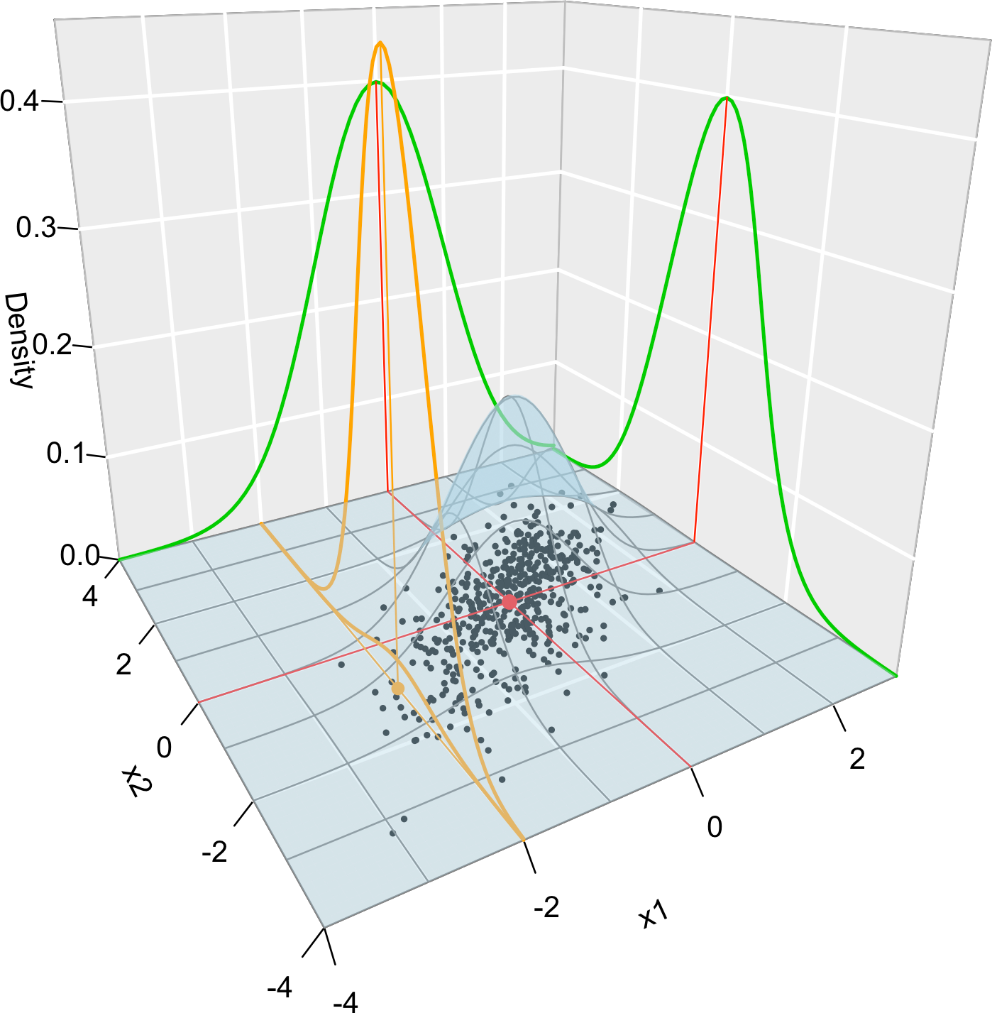
$Visualization of the joint pdf (in blue), marginal pdfs (green), conditional pdf of $X_2| X_1=x_1$ (orange), expectation (red point), and conditional expectation $\mathbb{E}\lbrack X_2 | X_1=x_1 \rbrack$ (orange point) of a $2$-dimensional normal. The conditioning point of $X_1$ is $x_1=-2.$ Note the different scales of the densities, as they have to integrate one over different supports. Note how the conditional density (upper orange curve) is not the joint pdf $f(x_1,x_2)$ (lower orange curve) with $x_1=-2$ but a rescaling of this curve by $\frac{1}{f_{X_1}(x_1)}.$ The parameters of the $2$-dimensional normal are $\mu_1=\mu_2=0,$ $\sigma_1=\sigma_2=1$ and $\rho=0.75.$ $500$ observations sampled from the distribution are shown in black.$

Figure 1.4: Visualization of the joint pdf (in blue), marginal pdfs (green), conditional pdf of $X_2| X_1=x_1$ (orange), expectation (red point), and conditional expectation $\mathbb{E}\lbrack X_2 | X_1=x_1 \rbrack$ (orange point) of a $2$ -dimensional normal. The conditioning point of $X_1$ is $x_1=-2.$ Note the different scales of the densities, as they have to integrate one over different supports. Note how the conditional density (upper orange curve) is not the joint pdf $f(x_1,x_2)$ (lower orange curve) with $x_1=-2$ but a rescaling of this curve by $\frac{1}{f_{X_1}(x_1)}.$ The parameters of the $2$ -dimensional normal are $\mu_1=\mu_2=0,$ $\sigma_1=\sigma_2=1$ and $\rho=0.75.$ $500$ observations sampled from the distribution are shown in black.

Finally, in the predictive models we will consider an independent and identically distributed (iid) sample of the response and the predictors. We use the following notation: $Y_i$ is the $i$ -th observation of the response $Y$ and $X_{ij}$ represents the $i$ -th observation of the $j$ -th predictor $X_j.$ Thus we will deal with samples of the form $\{(X_{i1},\ldots,X_{ip},Y_i)\}_{i=1}^n.$

Respectively, $F(x)=\int_{-\infty}^xf(t)\,\mathrm{d}t.$ ↩︎
The precise mathematical meaning of “ $\mathrm{d}F_X(x)$ ” is the Riemann–Stieltjes integral.↩︎
Understood as the probability that $(X_1\leq x_1)$ and $\ldots$ and $(X_p\leq x_p).$ ↩︎
Recall that the $X$ -part of $\mathbb{E}[Y| X]$ is random. However, $\mathbb{E}[Y| X=x]$ is deterministic.↩︎
If $\mu=0$ and $\sigma=1$ (standard normal), then the pdf and cdf are simply denoted by $\phi$ and $\Phi,$ without extra parameters.↩︎