4.1 Shrinkage

As we saw in Section 2.4.1, the least squares estimates \(\hat{\boldsymbol{\beta}}\) of the linear model

\[\begin{align*} Y = \beta_0 + \beta_1 X_1 + \cdots + \beta_p X_p + \varepsilon \end{align*}\]

were the minimizers of the residual sum of squares

\[\begin{align*} \text{RSS}(\boldsymbol{\beta})=\sum_{i=1}^n(Y_i-\beta_0-\beta_1X_{i1}-\cdots-\beta_pX_{ip})^2. \end{align*}\]

Under the validity of the assumptions of Section 2.3, in Section 2.4 we saw that

\[\begin{align*} \hat{\boldsymbol{\beta}}\sim\mathcal{N}_{p+1}\left(\boldsymbol{\beta},\sigma^2(\mathbf{X}'\mathbf{X})^{-1}\right). \end{align*}\]

A particular consequence of this result is that \(\hat{\boldsymbol{\beta}}\) is unbiased in estimating \(\boldsymbol{\beta},\) that is, \(\hat{\boldsymbol{\beta}}\) does not make any systematic error in estimating \(\boldsymbol{\beta}.\) However, bias is only one part of the quality of an estimate: variance is also important. Indeed, the bias-variance trade-off¹⁰³ arises from the bias-variance decomposition of the Mean Squared Error (MSE) of an estimate. For example, for the estimate \(\hat\beta_j\) of \(\beta_j,\) we have

\[\begin{align} \mathrm{MSE}[\hat\beta_j]:=\mathbb{E}[(\hat\beta_j-\beta_j)^2]=\underbrace{(\mathbb{E}[\hat\beta_j]-\beta_j)^2}_{\mathrm{Bias}^2}+\underbrace{\mathbb{V}\mathrm{ar}[\hat\beta_j]}_{\mathrm{Variance}}.\tag{4.1} \end{align}\]

Shrinkage methods pursue the following idea:

Add an amount of smart bias to \(\hat{\boldsymbol{\beta}}\) in order to reduce its variance, in such a way that we obtain simpler interpretations from the biased version of \(\hat{\boldsymbol{\beta}}.\)

This idea is implemented by enforcing sparsity, that is, by biasing the estimates of \(\boldsymbol{\beta}\) towards being non-null only for the most important predictors. The two main methods covered in this section, ridge regression and lasso (least absolute shrinkage and selection operator), use this idea in a different way. However, it is important to realize that both methods do consider the standard linear model; what they do different is the way of estimating \(\boldsymbol{\beta}\).

The way they enforce sparsity in the estimates is by minimizing the RSS plus a penalty term that favors sparsity on the estimated coefficients. For example, the ridge regression enforces a quadratic penalty to the candidate slope coefficients \(\boldsymbol\beta_{-1}=(\beta_1,\ldots,\beta_p)'\) and seeks to minimize¹⁰⁴

\[\begin{align} \text{RSS}(\boldsymbol{\beta})+\lambda\sum_{j=1}^p \beta_j^2=\text{RSS}(\boldsymbol{\beta})+\lambda\|\boldsymbol\beta_{-1}\|_2^2,\tag{4.2} \end{align}\]

where \(\lambda\geq 0\) is the penalty parameter. On the other hand, the lasso considers an absolute penalty:

\[\begin{align} \text{RSS}(\boldsymbol{\beta})+\lambda\sum_{j=1}^p |\beta_j|=\text{RSS}(\boldsymbol{\beta})+\lambda\|\boldsymbol\beta_{-1}\|_1.\tag{4.3} \end{align}\]

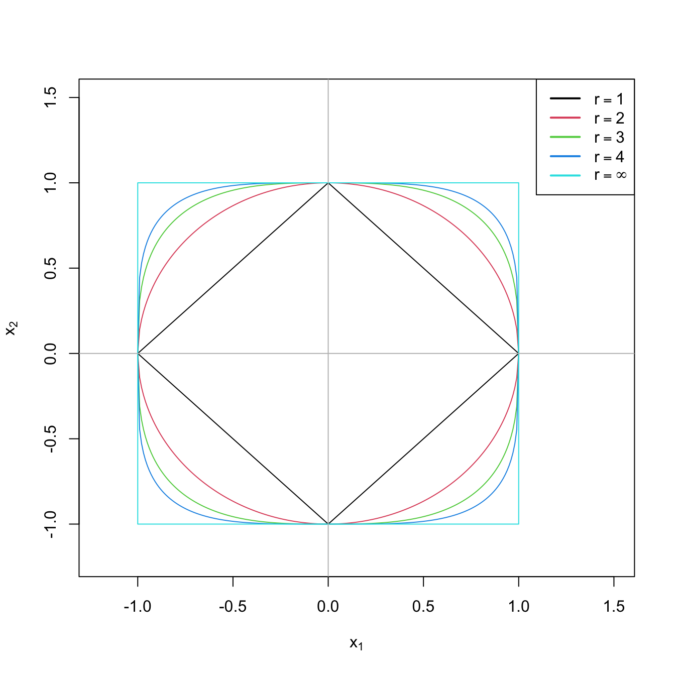
Figure 4.1: The “unit circle” \(\|(x_1,x_2)\|_r=1\) for \(r=1,2,3,4,\infty.\)

Among other possible joint representations for (4.2) and (4.3)¹⁰⁵, the one based on the elastic nets is particularly convenient, as it aims to combine the strengths of both methods in a computationally tractable way and is the one employed in the reference package glmnet. Considering a proportion \(0\leq\alpha\leq 1,\) the elastic net is defined as

\[\begin{align} \text{RSS}(\boldsymbol{\beta})+\lambda(\alpha\|\boldsymbol\beta_{-1}\|_1+(1-\alpha)\|\boldsymbol\beta_{-1}\|_2^2).\tag{4.4} \end{align}\]

Clearly, ridge regression corresponds to \(\alpha=0\) (quadratic penalty) and lasso to \(\alpha=1\) (absolute penalty). Obviously, if \(\lambda=0,\) we are back to the least squares problem and theory. The optimization of (4.4) gives

\[\begin{align} \hat{\boldsymbol{\beta}}_{\lambda,\alpha}:=\arg\min_{\boldsymbol{\beta}\in\mathbb{R}^{p+1}}\left\{ \text{RSS}(\boldsymbol{\beta})+\lambda\sum_{j=1}^p (\alpha|\beta_j|+(1-\alpha)|\beta_j|^2)\right\},\tag{4.5} \end{align}\]

which is the penalized estimation of \(\boldsymbol{\beta}.\) Note that the sparsity is enforced in the slopes, not in the intercept, since this depends on the mean of \(Y.\) Note also that the optimization problem is convex¹⁰⁶ and therefore it is guaranteed the existence and uniqueness of a minimum. However, in general¹⁰⁷, there are no explicit formulas for \(\hat{\boldsymbol{\beta}}_{\lambda,\alpha}\) and the optimization problem needs to be solved numerically. Finally, \(\lambda\) is a tuning parameter that will need to be chosen suitably and that we will discuss later¹⁰⁸. What it is important now is to recall that the predictors need to be standardized, or otherwise its scale will distort the optimization of (4.4).

An equivalent way of viewing (4.5) that helps in visualizing the differences between the ridge and lasso regressions is that they try to solve the equivalent optimization problem¹⁰⁹ of (4.5):

\[\begin{align} \hat{\boldsymbol{\beta}}_{s_\lambda,\alpha}:=\arg\min_{\boldsymbol{\beta}\in\mathbb{R}^{p+1}:\sum_{j=1}^p (\alpha|\beta_j|+(1-\alpha)|\beta_j|^2)\leq s_\lambda} \text{RSS}(\boldsymbol{\beta}),\tag{4.6} \end{align}\]

where \(s_\lambda\) is certain scalar that does not depend on \(\boldsymbol{\beta}.\)

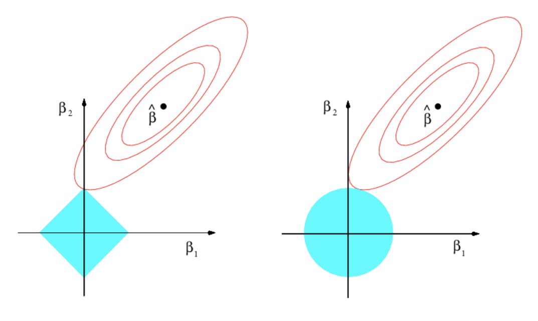
Figure 4.2: Comparison of ridge and lasso solutions from the optimization problem (4.6) with \(p=2.\) The elliptical contours show the regions with equal \(\mathrm{RSS}(\beta_1,\beta_2),\) the objective function, for \((\beta_1,\beta_2)\in\mathbb{R}^2\) (\(\beta_0=0\) is assumed). The diamond (\(\alpha=1\)) and circular (\(\alpha=0\)) regions show the feasibility regions determined by \(\sum_{j=1}^p (\alpha|\beta_j|+(1-\alpha)|\beta_j|^2)\leq s_\lambda\) for the optimization problem. The sharpness of the diamond makes the lasso attain solutions with many coefficients exactly equal to zero, in a similar situation to the one depicted. Extracted from James et al. (2013).

The glmnet package is the reference implementation of shrinkage estimators based on elastic nets. In order to illustrate how to apply the ridge and lasso regression in practice, we will work with the ISLR::Hitters dataset. This dataset contains statistics and salaries from baseball players from the 1986 and 1987 seasons. The objective will be to predict the Salary from the remaining predictors.

# Load data -- baseball players statistics
data(Hitters, package = "ISLR")

# Discard NA's
Hitters <- na.omit(Hitters)

# The glmnet function works with the design matrix of predictors (without
# the ones). This can be obtained easily through model.matrix()
x <- model.matrix(Salary ~ 0 + ., data = Hitters) 
# 0 + to exclude a column of 1's for the intercept, since the intercept will be 
# added by default in glmnet::glmnet and if we do not exclude it here we will 
# end with two intercepts, one of them resulting in NA. In the newer versions of
# glmnet this step is luckily not necessary

# Interestingly, note that in Hitters there are two-level factors and these
# are automatically transformed into dummy variables in x -- the main advantage 
# of model.matrix
head(Hitters[, 14:20])
##                   League Division PutOuts Assists Errors Salary NewLeague
## -Alan Ashby            N        W     632      43     10  475.0         N
## -Alvin Davis           A        W     880      82     14  480.0         A
## -Andre Dawson          N        E     200      11      3  500.0         N
## -Andres Galarraga      N        E     805      40      4   91.5         N
## -Alfredo Griffin       A        W     282     421     25  750.0         A
## -Al Newman             N        E      76     127      7   70.0         A
head(x[, 14:19])
##                   LeagueA LeagueN DivisionW PutOuts Assists Errors
## -Alan Ashby             0       1         1     632      43     10
## -Alvin Davis            1       0         1     880      82     14
## -Andre Dawson           0       1         0     200      11      3
## -Andres Galarraga       0       1         0     805      40      4
## -Alfredo Griffin        1       0         1     282     421     25
## -Al Newman              0       1         0      76     127      7

# We also need the vector of responses
y <- Hitters$Salary

model.matrix removes by default the observations with any NAs, returning only the complete cases. This may be undesirable in certain circumstances. If NAs are to be preserved, an option is to use na.action = "na.pass" but with the function model.matrix.lm (not model.matrix, as it ignores the argument!).

The next code illustrates the previous warning.

# Data with NA in the first observation
data_na <- data.frame("x1" = rnorm(3), "x2" = rnorm(3), "y" = rnorm(3))
data_na$x1[1] <- NA

# The first observation disappears!
model.matrix(y ~ 0 + ., data = data_na)
##           x1       x2
## 2  0.5136652 1.435410
## 3 -0.6558154 1.085212
## attr(,"assign")
## [1] 1 2

# Still ignores NA's
model.matrix(y ~ 0 + ., data = data_na, na.action = "na.pass")
##           x1       x2
## 2  0.5136652 1.435410
## 3 -0.6558154 1.085212
## attr(,"assign")
## [1] 1 2

# Does not ignore NA's
model.matrix.lm(y ~ 0 + ., data = data_na, na.action = "na.pass")
##           x1        x2
## 1         NA -1.329132
## 2  0.5136652  1.435410
## 3 -0.6558154  1.085212
## attr(,"assign")
## [1] 1 2

4.1.1 Ridge regression

We describe next how to do the fitting, tuning parameter selection, prediction, and the computation of the analytical form for the ridge regression. The first three topics are very similar for the lasso or for other elastic net fits (i.e., without \(\alpha=0\)).

Fitting

# Call to the main function -- use alpha = 0 for ridge regression
library(glmnet)
ridgeMod <- glmnet(x = x, y = y, alpha = 0)
# By default, it computes the ridge solution over a set of lambdas
# automatically chosen. It also standardizes the variables by default to make
# the model fitting since the penalization is scale-sensitive. Importantly,
# the coefficients are returned on the original scale of the predictors

# Plot of the solution path -- gives the value of the coefficients for different
# measures in xvar (penalization imposed to the model or fitness)
plot(ridgeMod, xvar = "norm", label = TRUE)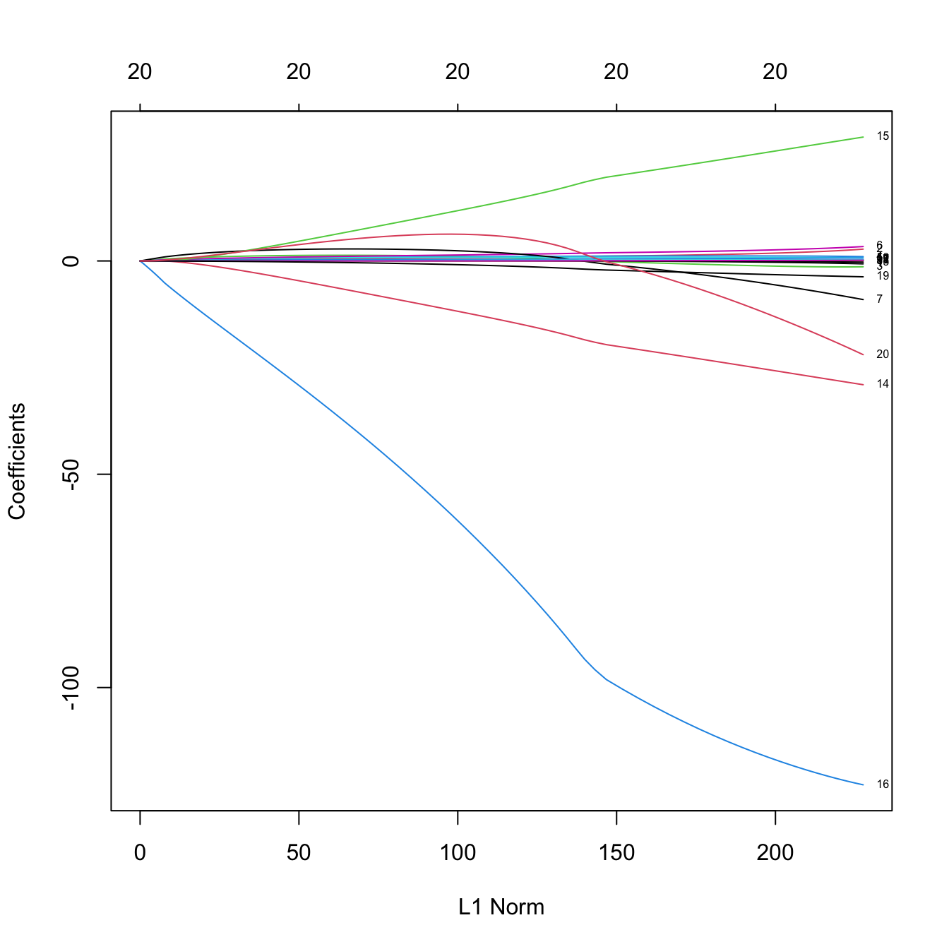

# xvar = "norm" is the default: L1 norm of the coefficients sum_j abs(beta_j)

# Versus lambda
plot(ridgeMod, label = TRUE, xvar = "lambda")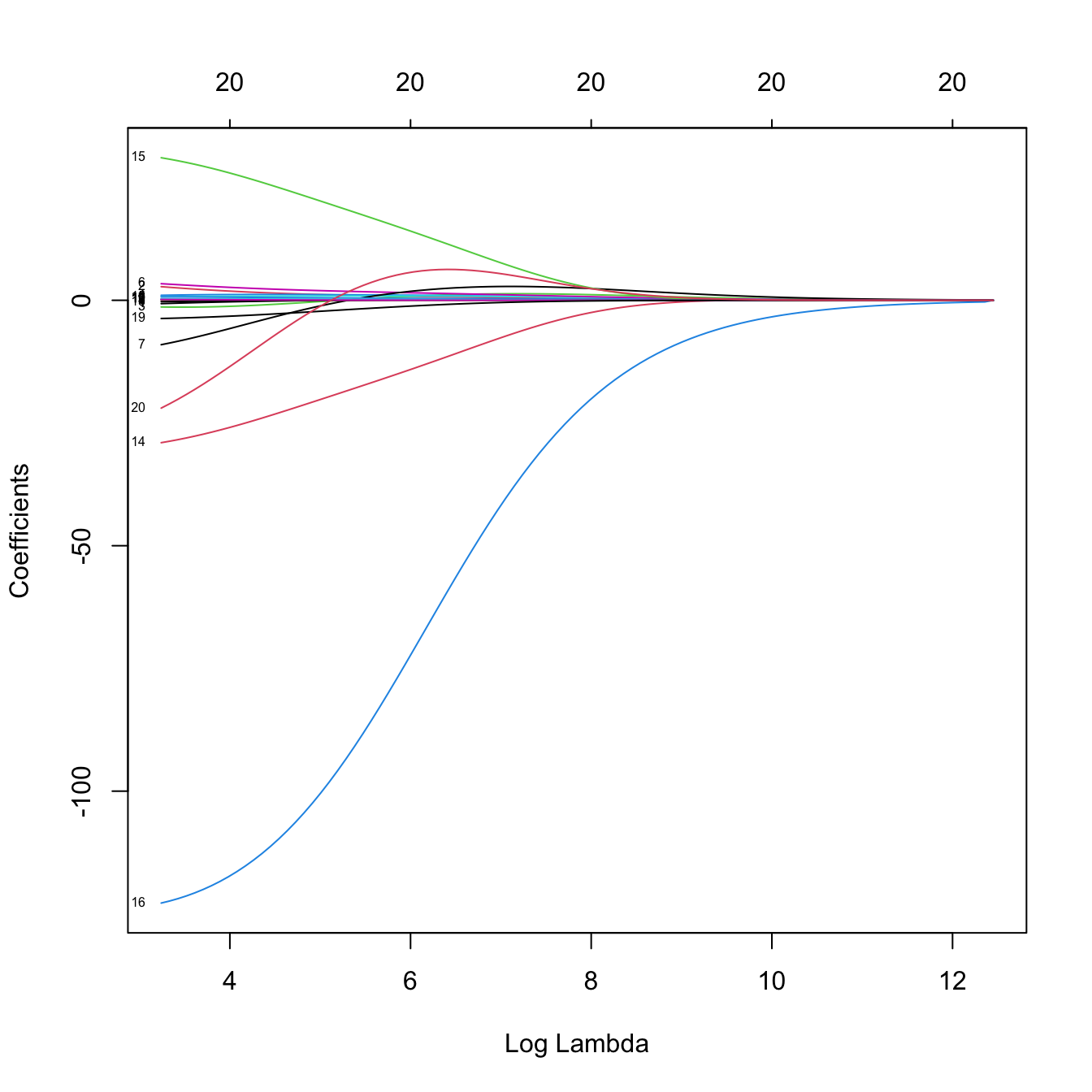

# Versus the percentage of deviance explained -- this is a generalization of the
# R^2 for generalized linear models. Since we have a linear model, this is the
# same as the R^2
plot(ridgeMod, label = TRUE, xvar = "dev")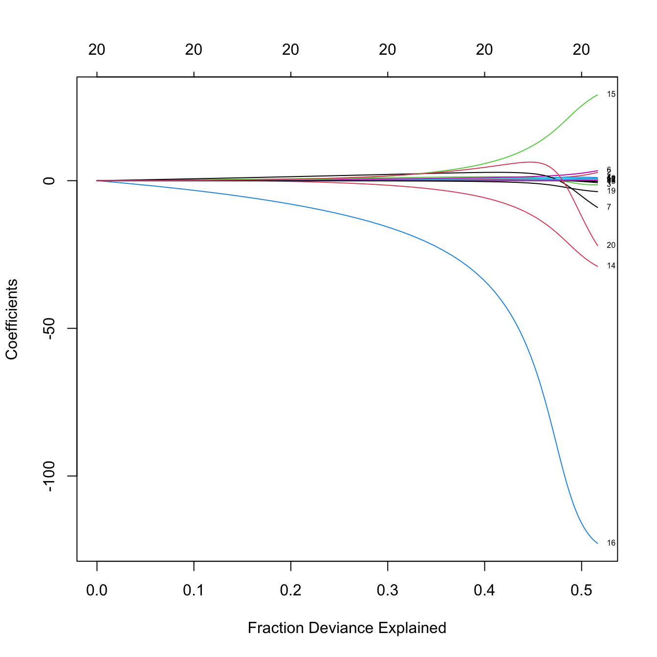

# The maximum R^2 is slightly above 0.5

# Indeed, we can see that R^2 = 0.5461
summary(lm(Salary ~., data = Hitters))$r.squared
## [1] 0.5461159

# Some persistently important predictors are 16, 14, and 15
colnames(x)[c(16, 14, 15)]
## [1] "DivisionW" "LeagueA"   "LeagueN"

# What is inside glmnet's output?
names(ridgeMod)
##  [1] "a0"        "beta"      "df"        "dim"       "lambda"    "dev.ratio" "nulldev"   "npasses"   "jerr"     
## [10] "offset"    "call"      "nobs"

# lambda versus R^2 -- fitness decreases when sparsity is introduced, in
# in exchange of better variable interpretation and avoidance of overfitting
plot(log(ridgeMod$lambda), ridgeMod$dev.ratio, type = "l",
     xlab = "log(lambda)", ylab = "R2")

ridgeMod$dev.ratio[length(ridgeMod$dev.ratio)]
## [1] 0.5164752
# Slightly different to lm's because it compromises accuracy for speed

# The coefficients for different values of lambda are given in $a0 (intercepts)
# and $beta (slopes) or, alternatively, both in coef(ridgeMod)
length(ridgeMod$a0)
## [1] 100
dim(ridgeMod$beta)
## [1]  20 100
length(ridgeMod$lambda) # 100 lambda's were automatically chosen
## [1] 100

# Inspecting the coefficients associated to the 50th lambda
coef(ridgeMod)[, 50]
##   (Intercept)         AtBat          Hits         HmRun          Runs           RBI         Walks         Years 
## 214.720400777   0.090210299   0.371622563   1.183305701   0.597288606   0.595291960   0.772639340   2.474046387 
##        CAtBat         CHits        CHmRun         CRuns          CRBI        CWalks       LeagueA       LeagueN 
##   0.007597343   0.029269640   0.217470479   0.058715486   0.060728347   0.058696981  -2.903863555   2.903558868 
##     DivisionW       PutOuts       Assists        Errors    NewLeagueN 
## -21.886726912   0.052629591   0.007406370  -0.147635449   2.663300534
ridgeMod$lambda[50]
## [1] 2674.375

# Zoom in path solution
plot(ridgeMod, label = TRUE, xvar = "lambda",
     xlim = log(ridgeMod$lambda[50]) + c(-2, 2), ylim = c(-30, 10))
abline(v = log(ridgeMod$lambda[50]))
points(rep(log(ridgeMod$lambda[50]), nrow(ridgeMod$beta)), ridgeMod$beta[, 50],
       pch = 16, col = 1:6)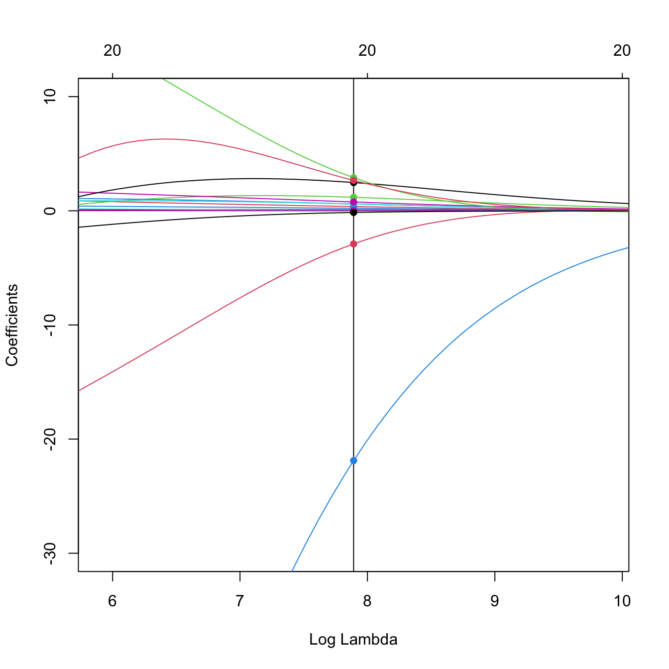

# The squared l2-norm of the coefficients decreases as lambda increases
plot(log(ridgeMod$lambda), sqrt(colSums(ridgeMod$beta^2)), type = "l",
     xlab = "log(lambda)", ylab = "l2 norm")

Tuning parameter selection

The selection of the penalty parameter \(\lambda\) is usually done by \(k\)-fold cross-validation, following the general principle described at the end of Section 3.6. This data-driven selector is denoted by \(\hat\lambda_{k\text{-CV}}\) and has the form given¹¹⁰ in (3.18) (or (3.17) if \(k=n\)):

\[\begin{align*} \hat{\lambda}_{k\text{-CV}}:=\arg\min_{\lambda\geq0} \text{CV}_k(\lambda),\quad \text{CV}_k(\lambda):=\sum_{j=1}^k \sum_{i\in F_j} (Y_i-\hat m_{\lambda,-F_{j}}(\mathbf{X}_i))^2. \end{align*}\]

A very interesting variant for the \(\hat{\lambda}_{k\text{-CV}}\) selector is the so-called one standard error rule. This rule is based on a parsimonious principle:

“favor simplicity within the set of most likely optimal models”.

It arises from observing that the objective function to minimize, \(\text{CV}_k,\) is random. Thus, its minimizer \(\hat{\lambda}_{k\text{-CV}}\) is subjected to variability. Then, the parsimonious approach proceeds by selecting not \(\hat{\lambda}_{k\text{-CV}},\) but the largest \(\lambda\) (hence, the simplest model) that is still likely optimal, i.e., that is “close” to \(\hat{\lambda}_{k\text{-CV}}.\) This closeness is quantified by the estimation of the standard deviation of the random variable \(\text{CV}_k(\hat\lambda_{k\text{-CV}}),\) which is obtained thanks to the folding splitting of the sample. Mathematically, \(\hat\lambda_{k\text{-1SE}}\) is defined as

\[\begin{align*} \hat\lambda_{k\text{-1SE}}:=\max\left\{\lambda\geq 0 : \text{CV}_k(\lambda)\in\left(\text{CV}_k(\hat\lambda_{k\text{-CV}})\pm\hat{\mathrm{SE}}\left(\text{CV}_k(\hat\lambda_{k\text{-CV}})\right)\right)\right\}. \end{align*}\]

The \(\hat\lambda_{k\text{-1SE}}\) selector often offers a good trade-off between model fitness and interpretability in practice.¹¹¹ The code below gives all the details.

# If we want, we can choose manually the grid of penalty parameters to explore
# The grid should be descending
ridgeMod2 <- glmnet(x = x, y = y, alpha = 0, lambda = 100:1)
plot(ridgeMod2, label = TRUE, xvar = "lambda") # Not a good choice!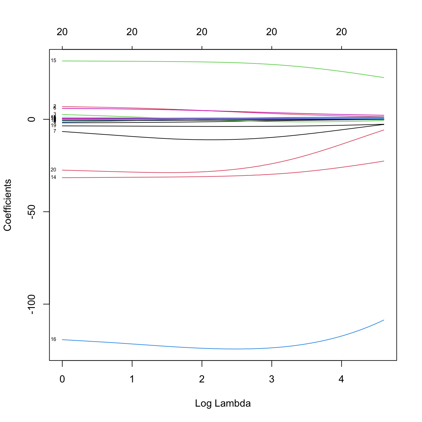

# Lambda is a tuning parameter that can be chosen by cross-validation, using as
# error the MSE (other possible error can be considered for generalized models
# using the argument type.measure)

# 10-fold cross-validation. Change the seed for a different result
set.seed(12345)
kcvRidge <- cv.glmnet(x = x, y = y, alpha = 0, nfolds = 10)

# The lambda that minimizes the CV error is
kcvRidge$lambda.min
## [1] 25.52821

# Equivalent to
indMin <- which.min(kcvRidge$cvm)
kcvRidge$lambda[indMin]
## [1] 25.52821

# The minimum CV error
kcvRidge$cvm[indMin]
## [1] 115034
min(kcvRidge$cvm)
## [1] 115034

# Potential problem! Minimum occurs at one extreme of the lambda grid in which
# CV is done. The grid was automatically selected, but can be manually inputted
range(kcvRidge$lambda)
## [1]     25.52821 255282.09651
lambdaGrid <- 10^seq(log10(kcvRidge$lambda[1]), log10(0.1),
                     length.out = 150) # log-spaced grid
kcvRidge2 <- cv.glmnet(x = x, y = y, nfolds = 10, alpha = 0,
                       lambda = lambdaGrid)

# Much better
plot(kcvRidge2)
kcvRidge2$lambda.min
## [1] 9.506186

# But the CV curve is random, since it depends on the sample. Its variability
# can be estimated by considering the CV curves of each fold. An alternative
# approach to select lambda is to choose the largest within one standard
# deviation of the minimum error, in order to favor simplicity of the model
# around the optimal lambda value. This is known as the "one standard error rule"
kcvRidge2$lambda.1se
## [1] 2964.928

# Location of both optimal lambdas in the CV loss function in dashed vertical
# lines, and lowest CV error and lowest CV error + one standard error
plot(kcvRidge2)
indMin2 <- which.min(kcvRidge2$cvm)
abline(h = kcvRidge2$cvm[indMin2] + c(0, kcvRidge2$cvsd[indMin2]))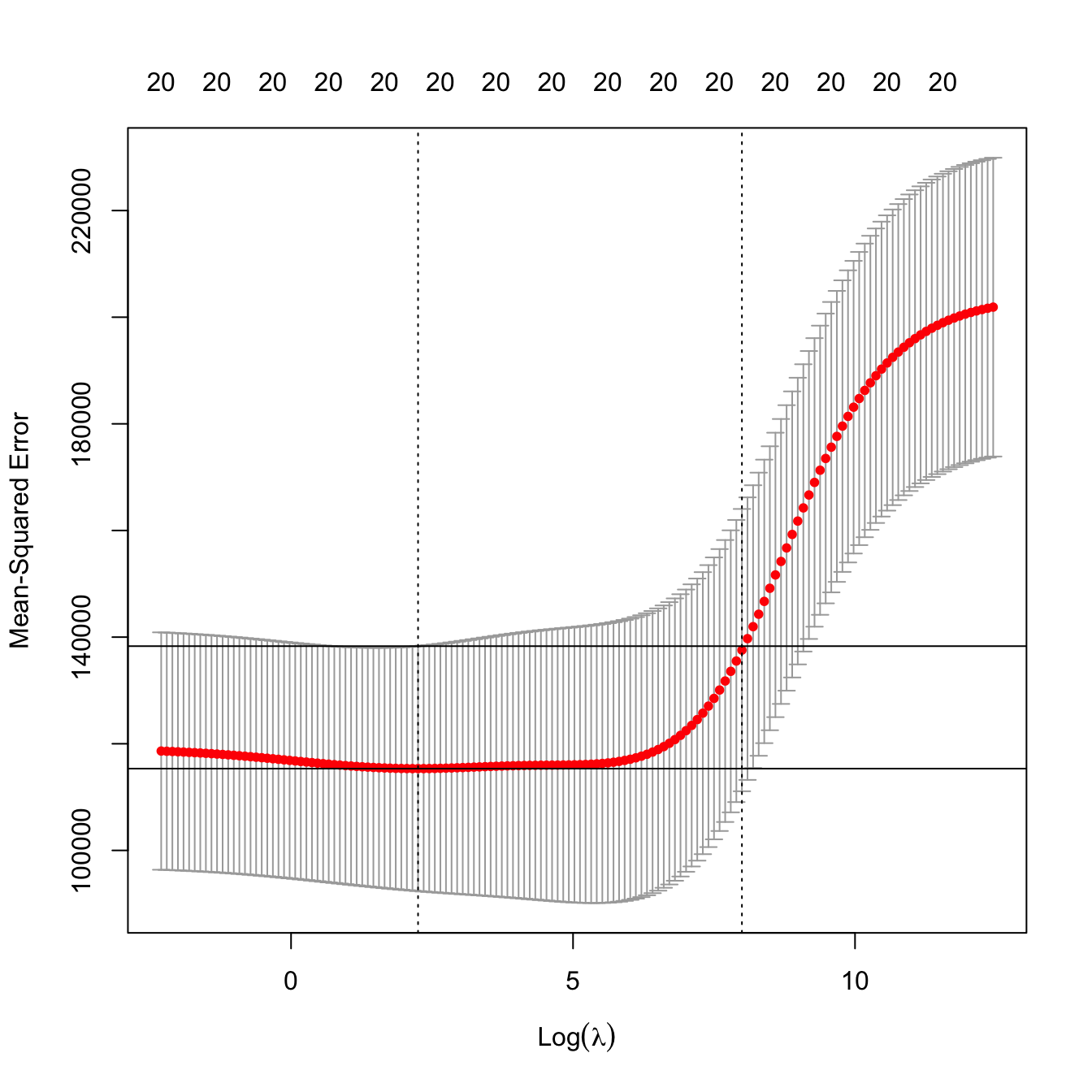

# The consideration of the one standard error rule for selecting lambda makes
# special sense when the CV function is quite flat around the minimum (hence an
# overpenalization that gives more sparsity does not affect so much the CV loss)

# Leave-one-out cross-validation. More computationally intense but completely
# objective in the choice of the fold-assignment
ncvRidge <- cv.glmnet(x = x, y = y, alpha = 0, nfolds = nrow(Hitters),
                      lambda = lambdaGrid)

# Location of both optimal lambdas in the CV loss function
plot(ncvRidge)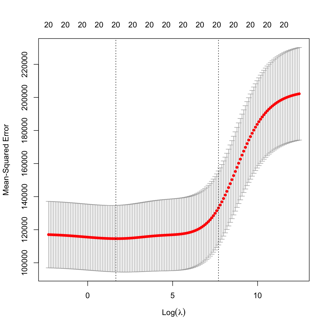

Prediction

# Inspect the best models (the glmnet fit is inside the output of cv.glmnet)
plot(kcvRidge2$glmnet.fit, label = TRUE, xvar = "lambda")
abline(v = log(c(kcvRidge2$lambda.min, kcvRidge2$lambda.1se)))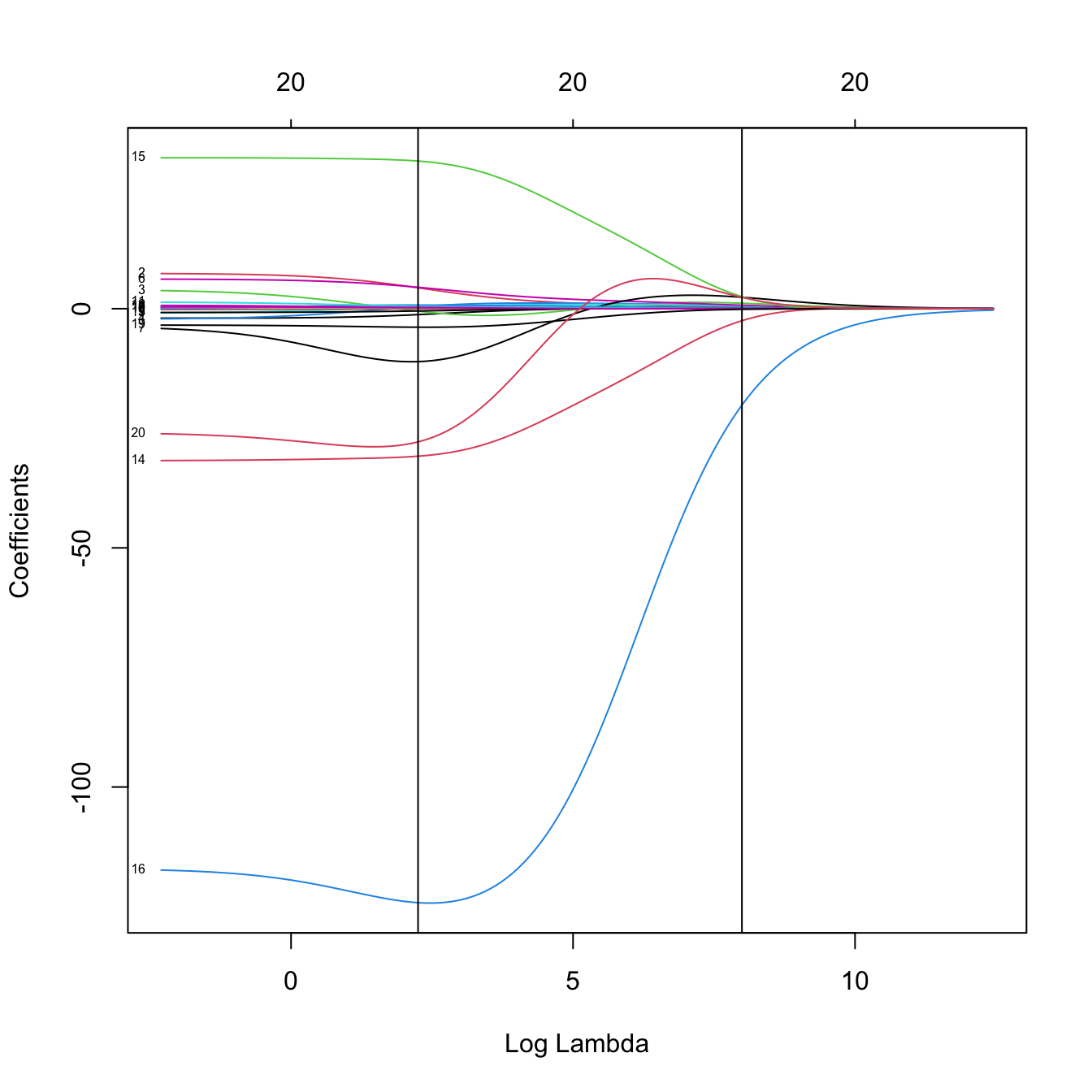

# The model associated to lambda.1se (or any other lambda not included in the
# original path solution -- obtained by an interpolation) can be retrieved with
predict(kcvRidge2, type = "coefficients", s = kcvRidge2$lambda.1se)
## 21 x 1 sparse Matrix of class "dgCMatrix"
##                        s1
## (Intercept) 229.758314334
## AtBat         0.086325740
## Hits          0.351303930
## HmRun         1.142772275
## Runs          0.567245068
## RBI           0.568056880
## Walks         0.731144713
## Years         2.389248929
## CAtBat        0.007261489
## CHits         0.027854683
## CHmRun        0.207220032
## CRuns         0.055877337
## CRBI          0.057777505
## CWalks        0.056352113
## LeagueA      -2.509251990
## LeagueN       2.509060248
## DivisionW   -20.162700810
## PutOuts       0.048911039
## Assists       0.006973696
## Errors       -0.128351187
## NewLeagueN    2.373103450

# Predictions for the first two observations
predict(kcvRidge2, type = "response", s = kcvRidge2$lambda.1se,
        newx = x[1:2, ])
##                    s1
## -Alan Ashby  530.8080
## -Alvin Davis 577.8485

# Predictions for the first observation, for all the lambdas. We can see how
# the prediction for one observation changes according to lambda
plot(log(kcvRidge2$lambda),
     predict(kcvRidge2, type = "response", newx = x[1, , drop = FALSE],
             s = kcvRidge2$lambda),
     type = "l", xlab = "log(lambda)", ylab = " Prediction")

Analytical form

The optimization problem (4.5) has an explicit solution for \(\alpha=0.\) To see it, assume that both the response \(Y\) and the predictors \(X_1,\ldots,X_p\) are centered, and that the sample \(\{(\mathbf{X}_i,Y_i)\}_{i=1}^n\) is also centered¹¹². In this case, there is no intercept \(\beta_0\) (\(=0\)) to estimate by \(\hat\beta_0\) (\(=0\)) and the linear model is simply

\[\begin{align*} Y=\beta_1X_1+\cdots+\beta_pX_p+\varepsilon. \end{align*}\]

Then, the ridge regression estimator \(\hat{\boldsymbol{\beta}}_{\lambda,0}\in\mathbb{R}^p\) is

\[\begin{align} \hat{\boldsymbol{\beta}}_{\lambda,0}&=\arg\min_{\boldsymbol{\beta}\in\mathbb{R}^{p}}\text{RSS}(\boldsymbol{\beta})+\lambda\|\boldsymbol\beta\|_2^2\nonumber\\ &=\arg\min_{\boldsymbol{\beta}\in\mathbb{R}^{p}}\sum_{i=1}^n(Y_i-\mathbf{X}_i\boldsymbol{\beta})^2+\lambda\boldsymbol\beta'\boldsymbol\beta\nonumber\\ &=\arg\min_{\boldsymbol{\beta}\in\mathbb{R}^{p}}(\mathbf{Y}-\mathbf{X}\boldsymbol{\beta})'(\mathbf{Y}-\mathbf{X}\boldsymbol{\beta})+\lambda\boldsymbol\beta'\boldsymbol\beta,\tag{4.7} \end{align}\]

where \(\mathbf{X}\) is the design matrix but now excluding the column of ones (thus of size \(n\times p\)). Nicely, (4.7) is a continuous quadratic optimization problem that is easily solved with the same arguments we employed for obtaining (2.7), resulting in¹¹³

\[\begin{align} \hat{\boldsymbol{\beta}}_{\lambda,0}=(\mathbf{X}'\mathbf{X}+\lambda\mathbf{I}_p)^{-1}\mathbf{X}'\mathbf{Y}.\tag{4.8} \end{align}\]

The form (4.8) neatly connects with the least squares estimator (\(\lambda=0\)) and yields many interesting insights. First, notice how the ridge regression estimator is always computable, even if \(p\gg n\;\)¹¹⁴ and the matrix \(\mathbf{X}'\mathbf{X}\) is not invertible, or if \(\mathbf{X}'\mathbf{X}\) is singular due to perfect multicollinearity. Second, as it was done with (2.11), it is straightforward to see that, under the assumptions of the linear model,

\[\begin{align} \hat{\boldsymbol{\beta}}_{\lambda,0}\sim\mathcal{N}_{p}\left((\mathbf{X}'\mathbf{X}+\lambda\mathbf{I}_p)^{-1}\mathbf{X}'\mathbf{X}\boldsymbol{\beta},\sigma^2(\mathbf{X}'\mathbf{X}+\lambda\mathbf{I}_p)^{-1}\mathbf{X}'\mathbf{X}(\mathbf{X}'\mathbf{X}+\lambda\mathbf{I}_p)^{-1}\right).\tag{4.9} \end{align}\]

The distribution (4.9) is revealing: it shows that \(\hat{\boldsymbol{\beta}}_{\lambda,0}\) is no longer unbiased and that its variance is smaller¹¹⁵ than the least squares estimator \(\hat{\boldsymbol{\beta}}.\) This is much more clear in the case where the predictors are uncorrelated and standardized, hence \(\mathbf{X}'\mathbf{X}=\mathbf{I}_p\) – precisely the case of the PCA or PLS scores if these are standardized to have unit variance. In this situation, then (4.8) and (4.9) simplify to

\[\begin{align} \begin{split} \hat{\boldsymbol{\beta}}_{\lambda,0}&=(1+\lambda)^{-1}\mathbf{X}'\mathbf{Y}=(1+\lambda)^{-1}\hat{\boldsymbol{\beta}},\\ \hat{\boldsymbol{\beta}}_{\lambda,0}&\sim\mathcal{N}_{p}\left((1+\lambda)^{-1}\boldsymbol{\beta},\sigma^2(1+\lambda)^{-2}\mathbf{I}_p\right). \end{split} \tag{4.10} \end{align}\]

The shrinking effect of \(\lambda\) is yet more evident from (4.10): when the predictors are uncorrelated, we shrink equally the least squares estimator \(\hat{\boldsymbol{\beta}}\) by the factor \((1+\lambda)^{-1},\) which results in a reduction of the variance by a factor of \((1+\lambda)^{-2}.\) Furthermore, notice an important point: due to the explicit control of the distribution of \(\hat{\boldsymbol{\beta}}_{\lambda,0},\) inference about \(\boldsymbol{\beta}\) can be done in a relatively straightforward¹¹⁶ way from \(\hat{\boldsymbol{\beta}}_{\lambda,0},\) just as it was done from \(\hat{\boldsymbol{\beta}}\) in Section 2.4. This tractability, both on the explicit form of the estimator and on the associated inference, is one of the main advantages of ridge regression with respect to other shrinkage methods.

Finally, just as we did for the least squares estimator, we can define the hat matrix

\[\begin{align*} \mathbf{H}_\lambda:=\mathbf{X}(\mathbf{X}'\mathbf{X}+\lambda\mathbf{I}_p)^{-1}\mathbf{X}' \end{align*}\]

that predicts \(\hat{\mathbf{Y}}\) from \(\mathbf{Y}.\) This hat matrix becomes especially useful now, as it can be employed to define the effective degrees of freedom associated to a ridge regression with penalty \(\lambda.\) These are defined as the trace of the hat matrix:

\[\begin{align*} \mathrm{df}(\lambda):=\mathrm{tr}(\mathbf{H}_\lambda). \end{align*}\]

The motivation behind is that, for the unrestricted least squares fit¹¹⁷

\[\begin{align*} \mathrm{tr}(\mathbf{H}_0)=\mathrm{tr}\big(\mathbf{X}(\mathbf{X}'\mathbf{X})^{-1}\mathbf{X}'\big)=\mathrm{tr}\big(\mathbf{X}'\mathbf{X}(\mathbf{X}'\mathbf{X})^{-1}\big)=p \end{align*}\]

and thus indeed \(\mathrm{df}(0)=p\) is representing the degrees of freedom of the fit, understood as the number of parameters employed (keep in mind that the intercept was excluded). For a constrained fit with \(\lambda>0,\) \(\mathrm{df}(\lambda)<p\) because, even if we are estimating \(p\) parameters in \(\hat{\boldsymbol{\beta}}_{\lambda,0},\) these are restricted to satisfy \(\|\hat{\boldsymbol{\beta}}_{\lambda,0}\|^2_2\leq s_\lambda\) (for a certain \(s_\lambda,\) recall (4.6)). The function \(\mathrm{df}\) is monotonically decreasing and such that \(\lim_{\lambda\to\infty}\mathrm{df}(\lambda)=0,\) see Figure 4.3. Recall that, due to the imposed constraint on the coefficients, we could choose \(\lambda\) such that \(\mathrm{df}(\lambda)=r,\) where \(r\) is an integer smaller than \(p\): this would correspond to effectively employing exactly \(r\) parameters in the regression, despite considering \(p\) predictors.

Figure 4.3: The effective degrees of freedom \(\mathrm{df}(\lambda)\) as a function of \(\log(\lambda)\) for a ridge regression with \(p=5.\)

The next chunk of code implements \(\hat{\boldsymbol{\beta}}_{\lambda,0}\) and shows that is equivalent to the output of glmnet::glmnet, with certain quirks¹¹⁸.

# Random data
p <- 5
n <- 200
beta <- seq(-1, 1, l = p)
set.seed(123124)
x <- matrix(rnorm(n * p), n, p)
y <- 1 + x %*% beta + rnorm(n)

# Unrestricted fit
fit <- glmnet(x, y, alpha = 0, lambda = 0, intercept = TRUE, 
              standardize = FALSE)
beta0Hat <- rbind(fit$a0, fit$beta)
beta0Hat
## 6 x 1 sparse Matrix of class "dgCMatrix"
##             s0
##     1.05856208
## V1 -1.03109958
## V2 -0.56932123
## V3 -0.03813426
## V4  0.47415412
## V5  1.05761841

# Unrestricted fit matches least squares -- but recall glmnet uses an
# iterative method so it is inexact (convergence threshold thresh = 1e-7 by 
# default)
X <- model.matrix(y ~ x) # A way of constructing a design matrix that is a
# data.frame and has a column of ones
solve(crossprod(X)) %*% t(X) %*% y
##                    [,1]
## (Intercept)  1.05856209
## x1          -1.03109954
## x2          -0.56932123
## x3          -0.03813426
## x4           0.47415412
## x5           1.05761841

# Restricted fit
# glmnet considers as the regularization parameter "lambda" the value
# lambda / n (lambda being here the penalty parameter employed in the theory)
lambda <- 2
fit <- glmnet(x, y, alpha = 0, lambda = lambda / n, intercept = TRUE,
              standardize = FALSE)
betaLambdaHat <- rbind(fit$a0, fit$beta)
betaLambdaHat
## 6 x 1 sparse Matrix of class "dgCMatrix"
##            s0
##     1.0586029
## V1 -1.0264951
## V2 -0.5667469
## V3 -0.0377357
## V4  0.4710700
## V5  1.0528297

# Analytical form with intercept
solve(crossprod(X) + diag(c(0, rep(lambda, p)))) %*% t(X) %*% y
##                    [,1]
## (Intercept)  1.05864278
## x1          -1.02203900
## x2          -0.56425607
## x3          -0.03735258
## x4           0.46809435
## x5           1.04819600

4.1.2 Lasso

The main novelty in lasso with respect to ridge is its ability to exactly zeroing coefficients and the lack of analytical solution. Fitting, tuning parameter selection, and prediction are completely analogous to ridge regression.

Fitting

# Get the Hitters data back
x <- model.matrix(Salary ~ 0 + ., data = Hitters) 
y <- Hitters$Salary

# Call to the main function -- use alpha = 1 for lasso regression (the default)
lassoMod <- glmnet(x = x, y = y, alpha = 1)
# Same defaults as before, same object structure

# Plot of the solution path -- now the paths are not smooth when decreasing to
# zero (they are zero exactly). This is a consequence of the l1 norm
plot(lassoMod, xvar = "lambda", label = TRUE)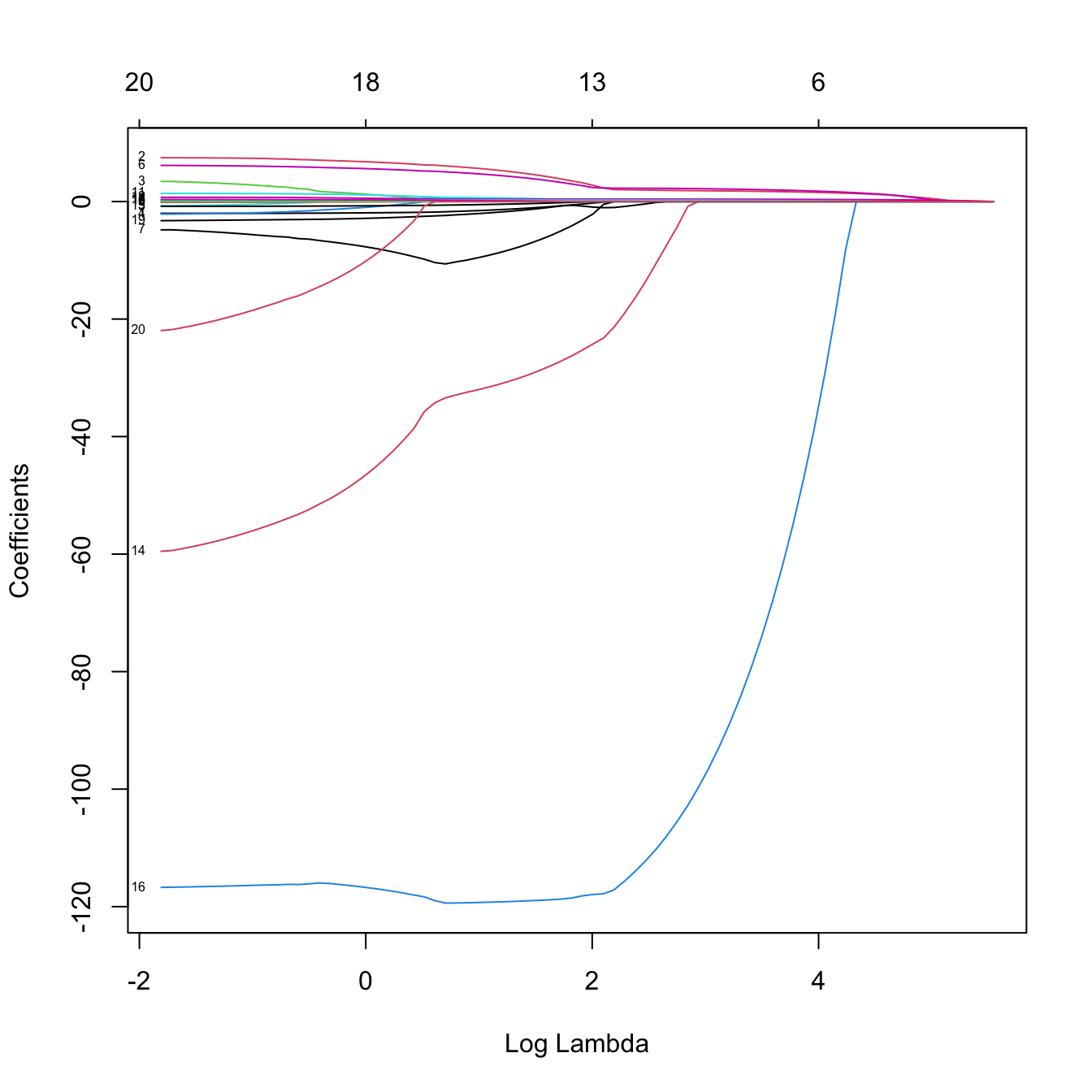

# Some persistently important predictors are 16 and 14

# Versus the R^2 -- same maximum R^2 as before
plot(lassoMod, label = TRUE, xvar = "dev")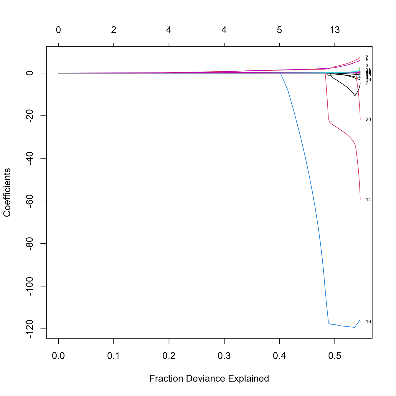

# Now the l1-norm of the coefficients decreases as lambda increases
plot(log(lassoMod$lambda), colSums(abs(lassoMod$beta)), type = "l",
     xlab = "log(lambda)", ylab = "l1 norm")

# 10-fold cross-validation. Change the seed for a different result
set.seed(12345)
kcvLasso <- cv.glmnet(x = x, y = y, alpha = 1, nfolds = 10)

# The lambda that minimizes the CV error
kcvLasso$lambda.min
## [1] 2.674375

# The "one standard error rule" for lambda
kcvLasso$lambda.1se
## [1] 76.16717

# Location of both optimal lambdas in the CV loss function
indMin <- which.min(kcvLasso$cvm)
plot(kcvLasso)
abline(h = kcvLasso$cvm[indMin] + c(0, kcvLasso$cvsd[indMin]))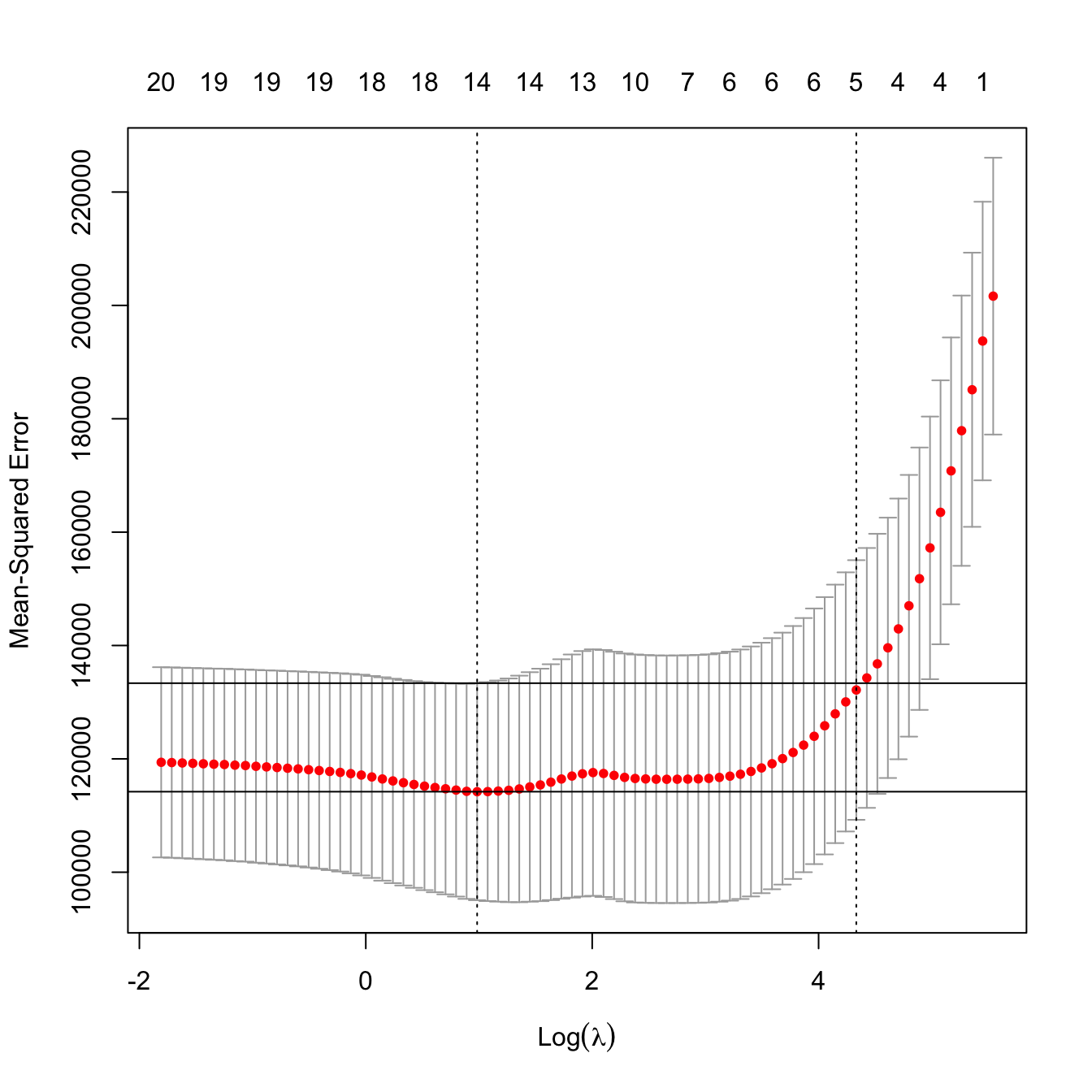

# No problems now: the minimum does not occur at one extreme
# Interesting: note that the numbers on top of the figure give the number of
# coefficients *exactly* different from zero -- the number of predictors
# effectively considered in the model!
# In this case, the one standard error rule makes also sense

# Leave-one-out cross-validation
lambdaGrid <- 10^seq(log10(kcvLasso$lambda[1]), log10(0.1),
                     length.out = 150) # log-spaced grid
ncvLasso <- cv.glmnet(x = x, y = y, alpha = 1, nfolds = nrow(Hitters),
                      lambda = lambdaGrid)

# Location of both optimal lambdas in the CV loss function
plot(ncvLasso)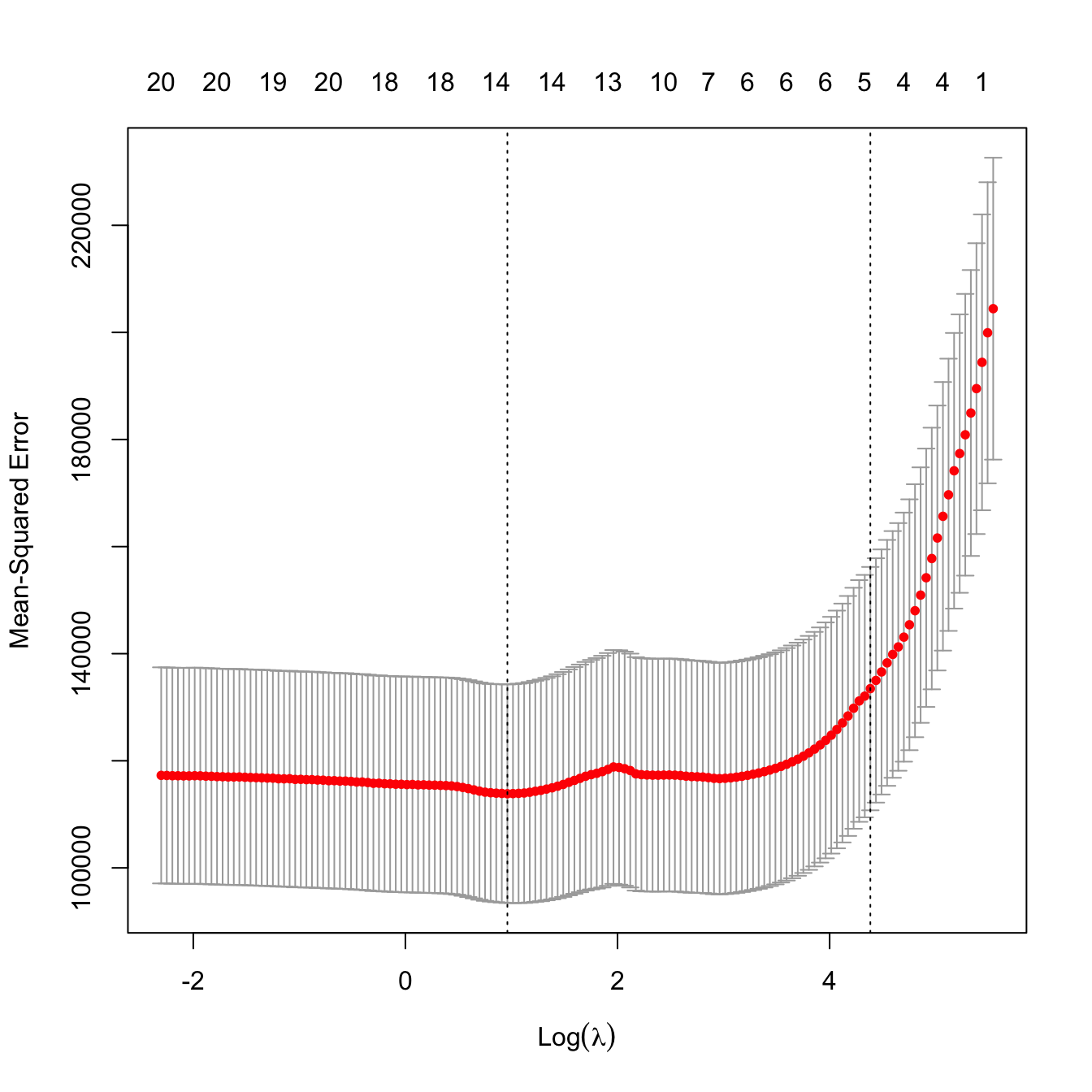

Prediction

# Inspect the best models
plot(kcvLasso$glmnet.fit, label = TRUE, xvar = "lambda")
abline(v = log(c(kcvLasso$lambda.min, kcvLasso$lambda.1se)))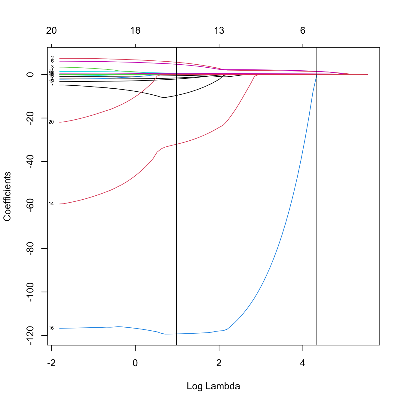

# The model associated to lambda.min (or any other lambda not included in the
# original path solution -- obtained by an interpolation) can be retrieved with
predict(kcvLasso, type = "coefficients",
        s = c(kcvLasso$lambda.min, kcvLasso$lambda.1se))
## 21 x 2 sparse Matrix of class "dgCMatrix"
##                        s1           s2
## (Intercept)  1.558172e+02 144.37970458
## AtBat       -1.547343e+00   .         
## Hits         5.660897e+00   1.36380384
## HmRun        .              .         
## Runs         .              .         
## RBI          .              .         
## Walks        4.729691e+00   1.49731098
## Years       -9.595837e+00   .         
## CAtBat       .              .         
## CHits        .              .         
## CHmRun       5.108207e-01   .         
## CRuns        6.594856e-01   0.15275165
## CRBI         3.927505e-01   0.32833941
## CWalks      -5.291586e-01   .         
## LeagueA     -3.206508e+01   .         
## LeagueN      2.108435e-12   .         
## DivisionW   -1.192990e+02   .         
## PutOuts      2.724045e-01   0.06625755
## Assists      1.732025e-01   .         
## Errors      -2.058508e+00   .         
## NewLeagueN   .              .

# Predictions for the first two observations
predict(kcvLasso, type = "response",
        s = c(kcvLasso$lambda.min, kcvLasso$lambda.1se),
        newx = x[1:2, ])
##                    s1       s2
## -Alan Ashby  427.8822 540.0835
## -Alvin Davis 700.1705 615.3311

4.1.3 Variable selection with lasso

Thanks to its ability to exactly zeroing coefficients, lasso is a powerful device for performing variable/model selection within its fit. The practical approach is really simple and amounts to identify the entries of \(\hat{\boldsymbol{\beta}}_{\lambda,1}\) different from zero, after \(\lambda\) is appropriately selected.

# We can use lasso for model selection!
selPreds <- predict(kcvLasso, type = "coefficients",
                    s = c(kcvLasso$lambda.min, kcvLasso$lambda.1se))[-1, ] != 0
x1 <- x[, selPreds[, 1]]
x2 <- x[, selPreds[, 2]]

# Least squares fit with variables selected by lasso
modLassoSel1 <- lm(y ~ x1)
modLassoSel2 <- lm(y ~ x2)
summary(modLassoSel1)
## 
## Call:
## lm(formula = y ~ x1)
## 
## Residuals:
##     Min      1Q  Median      3Q     Max 
## -940.10 -174.20  -25.94  127.05 1890.12 
## 
## Coefficients: (1 not defined because of singularities)
##               Estimate Std. Error t value Pr(>|t|)    
## (Intercept)  224.24408   84.45013   2.655 0.008434 ** 
## x1AtBat       -2.30798    0.56236  -4.104  5.5e-05 ***
## x1Hits         7.34602    1.71760   4.277  2.7e-05 ***
## x1Walks        6.08610    1.57008   3.876 0.000136 ***
## x1Years      -13.60502   10.38333  -1.310 0.191310    
## x1CHmRun       0.83633    0.84709   0.987 0.324457    
## x1CRuns        0.90924    0.27662   3.287 0.001159 ** 
## x1CRBI         0.35734    0.36252   0.986 0.325229    
## x1CWalks      -0.83918    0.27207  -3.084 0.002270 ** 
## x1LeagueA    -36.68460   40.73468  -0.901 0.368685    
## x1LeagueN           NA         NA      NA       NA    
## x1DivisionW -119.67399   39.32485  -3.043 0.002591 ** 
## x1PutOuts      0.29296    0.07632   3.839 0.000157 ***
## x1Assists      0.31483    0.20460   1.539 0.125142    
## x1Errors      -3.23219    4.29443  -0.753 0.452373    
## ---
## Signif. codes:  0 '***' 0.001 '**' 0.01 '*' 0.05 '.' 0.1 ' ' 1
## 
## Residual standard error: 314 on 249 degrees of freedom
## Multiple R-squared:  0.5396, Adjusted R-squared:  0.5156 
## F-statistic: 22.45 on 13 and 249 DF,  p-value: < 2.2e-16
summary(modLassoSel2)
## 
## Call:
## lm(formula = y ~ x2)
## 
## Residuals:
##     Min      1Q  Median      3Q     Max 
## -914.21 -171.94  -33.26   97.63 2197.08 
## 
## Coefficients:
##              Estimate Std. Error t value Pr(>|t|)    
## (Intercept) -96.96096   55.62583  -1.743 0.082513 .  
## x2Hits        2.09338    0.57376   3.649 0.000319 ***
## x2Walks       2.51513    1.22010   2.061 0.040269 *  
## x2CRuns       0.26490    0.19463   1.361 0.174679    
## x2CRBI        0.39549    0.19755   2.002 0.046339 *  
## x2PutOuts     0.26620    0.07857   3.388 0.000814 ***
## ---
## Signif. codes:  0 '***' 0.001 '**' 0.01 '*' 0.05 '.' 0.1 ' ' 1
## 
## Residual standard error: 333 on 257 degrees of freedom
## Multiple R-squared:  0.4654, Adjusted R-squared:  0.455 
## F-statistic: 44.75 on 5 and 257 DF,  p-value: < 2.2e-16

# Comparison with stepwise selection
modBIC <- MASS::stepAIC(lm(Salary ~ ., data = Hitters), k = log(nrow(Hitters)),
                        trace = 0)
summary(modBIC)
## 
## Call:
## lm(formula = Salary ~ AtBat + Hits + Walks + CRuns + CRBI + CWalks + 
##     Division + PutOuts, data = Hitters)
## 
## Residuals:
##     Min      1Q  Median      3Q     Max 
## -794.06 -171.94  -28.48  133.36 2017.83 
## 
## Coefficients:
##               Estimate Std. Error t value Pr(>|t|)    
## (Intercept)  117.15204   65.07016   1.800 0.072985 .  
## AtBat         -2.03392    0.52282  -3.890 0.000128 ***
## Hits           6.85491    1.65215   4.149 4.56e-05 ***
## Walks          6.44066    1.52212   4.231 3.25e-05 ***
## CRuns          0.70454    0.24869   2.833 0.004981 ** 
## CRBI           0.52732    0.18861   2.796 0.005572 ** 
## CWalks        -0.80661    0.26395  -3.056 0.002483 ** 
## DivisionW   -123.77984   39.28749  -3.151 0.001824 ** 
## PutOuts        0.27539    0.07431   3.706 0.000259 ***
## ---
## Signif. codes:  0 '***' 0.001 '**' 0.01 '*' 0.05 '.' 0.1 ' ' 1
## 
## Residual standard error: 314.7 on 254 degrees of freedom
## Multiple R-squared:  0.5281, Adjusted R-squared:  0.5133 
## F-statistic: 35.54 on 8 and 254 DF,  p-value: < 2.2e-16
# The lasso variable selection is similar, although the model is slightly worse
# in terms of adjusted R^2 and significance of the predictors. However, keep in
# mind that lasso is solving a constrained least squares problem, so it is
# expected to achieve better R^2 and adjusted R^2 via a selection procedure
# that employs solutions of unconstrained least squares. What is remarkable
# is the speed of lasso on selecting variables, and the fact that gives quite
# good starting points for performing further model selection

# Another interesting possibility is to run a stepwise selection starting from
# the set of predictors selected by lasso. In this search, it is important to
# use direction = "both" (default) and define the scope argument adequately
f <- formula(paste("Salary ~", paste(names(which(selPreds[, 2])), 
                                     collapse = " + ")))
start <- lm(f, data = Hitters) # Model with predictors selected by lasso
scope <- list(lower = lm(Salary ~ 1, data = Hitters), # No predictors
              upper = lm(Salary ~ ., data = Hitters)) # All the predictors
modBICFromLasso <- MASS::stepAIC(object = start, k = log(nrow(Hitters)),
                                 scope = scope, trace = 0)
summary(modBICFromLasso)
## 
## Call:
## lm(formula = Salary ~ Hits + Walks + CRBI + PutOuts + AtBat + 
##     Division, data = Hitters)
## 
## Residuals:
##     Min      1Q  Median      3Q     Max 
## -873.11 -181.72  -25.91  141.77 2040.47 
## 
## Coefficients:
##               Estimate Std. Error t value Pr(>|t|)    
## (Intercept)   91.51180   65.00006   1.408 0.160382    
## Hits           7.60440    1.66254   4.574 7.46e-06 ***
## Walks          3.69765    1.21036   3.055 0.002488 ** 
## CRBI           0.64302    0.06443   9.979  < 2e-16 ***
## PutOuts        0.26431    0.07477   3.535 0.000484 ***
## AtBat         -1.86859    0.52742  -3.543 0.000470 ***
## DivisionW   -122.95153   39.82029  -3.088 0.002239 ** 
## ---
## Signif. codes:  0 '***' 0.001 '**' 0.01 '*' 0.05 '.' 0.1 ' ' 1
## 
## Residual standard error: 319.9 on 256 degrees of freedom
## Multiple R-squared:  0.5087, Adjusted R-squared:  0.4972 
## F-statistic: 44.18 on 6 and 256 DF,  p-value: < 2.2e-16

# Comparison in terms of BIC, slight improvement with modBICFromLasso
BIC(modLassoSel1, modLassoSel2, modBICFromLasso, modBIC)
##                 df      BIC
## modLassoSel1    15 3839.690
## modLassoSel2     7 3834.434
## modBICFromLasso  8 3817.785
## modBIC          10 3818.320

Consider la-liga-2015-2016.xlsx dataset. We aim to predict Points after removing the perfectly related linear variables with Points. Do the following:

1. Lasso regression. Select \(\lambda\) by cross-validation. Obtain the estimated coefficients for the chosen lambda.
2. Use the predictors with non-null coefficients for creating a model with lm.
3. Summarize the model and check for multicollinearity.

It may happen that the cross-validation curve has an “L”-shaped form without a well-defined global minimum. This usually happens when only the intercept is significative and none of the predictors are relevant for explaining \(Y.\)

The code below illustrates the previous warning.

# Random data with predictors unrelated with the response
p <- 100
n <- 300
set.seed(123124)
x <- matrix(rnorm(n * p), n, p)
y <- 1 + rnorm(n)

# CV
lambdaGrid <- exp(seq(-10, 3, l = 200))
plot(cv.glmnet(x = x, y = y, alpha = 1, nfolds = n, lambda = lambdaGrid))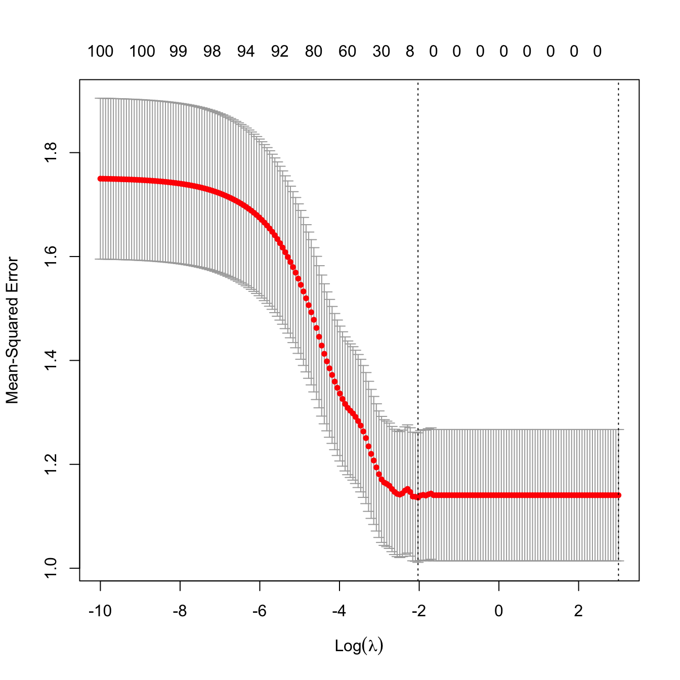

Figure 4.4: “L”-shaped form of a cross-validation curve with unrelated response and predictors.

The lasso-selection of variables is conceptually and practically straightforward. But, is this a consistent model selection procedure? As seen in Section 3.2.2, the answer to this question may be sometimes surprising and may have important practical consequences.

Zhao and Yu (2006) proved that lasso is consistent on the selection of the true model¹¹⁹ if a certain condition, known as the strong irrepresentable condition, holds for the predictors. It is also required that the regularization parameter \(\lambda\equiv \lambda_n\) is such that \(\lambda_n \to0,\) at some specific speeds¹²⁰, as \(n\to\infty.\) The strong irrepresentable condition is quite technical, but essentially is satisfied if the correlations between the predictors are appropriately controlled. In particular, Zhao and Yu (2006) identify several simple situations for the predictors that guarantee that the strong irrepresentable condition holds:

• If the predictors are uncorrelated.
• If the correlations of the predictors are bounded by a certain constant. Precisely, if \(\boldsymbol{\beta}_{-1}\) has \(q\) entries different from zero, it must be satisfied that \(\mathrm{Cor}[X_i,X_j]\leq \frac{c}{2q-1}\) for a constant \(0\leq c< 1,\) for all \(i,j=1,\ldots,p,\) \(i\neq j.\)¹²¹
• If the correlations of the predictors are power-decaying. That is, if \(\mathrm{Cor}[X_i,X_j]=\rho^{|i-j|},\) for \(|\rho|<1\) and for all \(i,j=1,\ldots,p.\)

Despite the usefulness of these three conditions, they do not inform directly on the consistency of the lasso in the more complex situation in which a data-driven penalizing parameter \(\hat{\lambda}\) is used (as opposed to a deterministic sequence \(\lambda_n\to0,\) as in Zhao and Yu (2006)). Let’s explore this situation by retaking the simulation study behind Figure 3.5. Within the same settings described there, we lasso-select the predictors with estimated coefficients different from zero using \(\hat{\lambda}_{n\text{-CV}}\) and \(\hat\lambda_{n\text{-1SE}},\) then approximate by Monte Carlo the probability of selecting the true model. The results are collected in Figure 4.5.

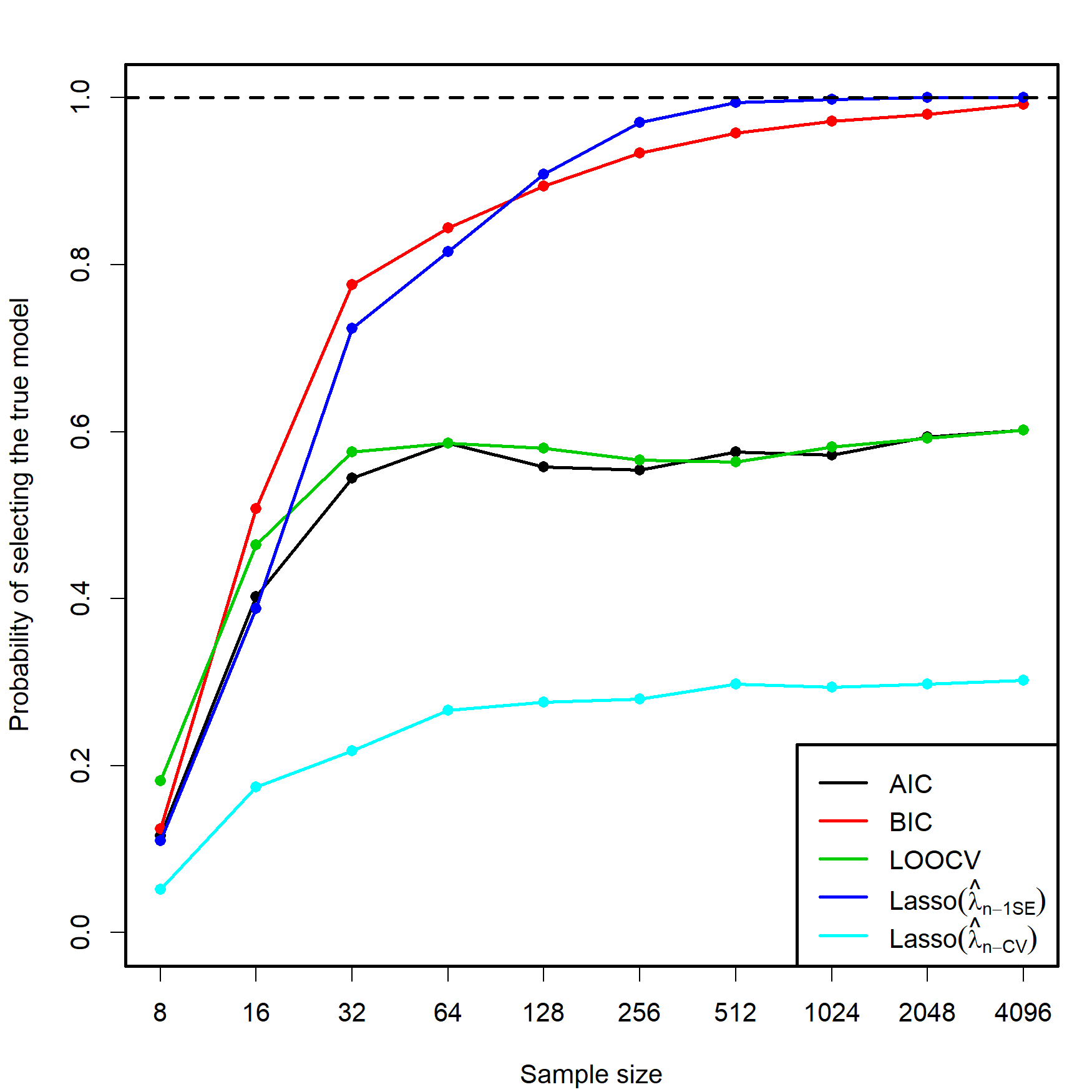
Figure 4.5: Estimation of the probability of selecting the correct model by lasso selection based on \(\hat{\lambda}_{n\text{-CV}}\) and \(\hat\lambda_{n\text{-1SE}},\) and by minimizing the AIC, BIC, and LOOCV criteria in an exhaustive search (see Figure 3.5). There are \(p=5\) independent predictors and the correct model contained two predictors. The probability was estimated with \(M=500\) Monte Carlo runs.

In addition to the insights from Figure 3.5, Figure 4.5 shows interesting results, described next. Recall that the simulation study was performed with independent predictors.

• Lasso-selection based on \(\hat{\lambda}_{n\text{-CV}}\) is inconsistent. It tends to select more predictors than required, as AIC does, yet its performance is much worse (about a \(0.25\) probability of recovering the true model!). This result is somehow coherent what it would be expected from Shao (1993)’s result on the inconsistency of LOOCV.
• Lasso-selection based on \(\hat\lambda_{n\text{-1SE}}\) seems to be¹²² consistent and imitates the performance of the BIC¹²³. Observe that the overpenalization given by the one standard error rule somehow resembles the overpenalization of BIC with respect to AIC.

Implement the lasso part of the simulation study behind Figure 4.5:

1. Sample from (3.4).
2. Compute the \(\hat{\lambda}_{n\text{-CV}}\) and \(\hat\lambda_{n\text{-1SE}}.\)
3. Identify the estimated coefficients for \(\hat{\lambda}_{n\text{-CV}}\) and \(\hat\lambda_{n\text{-1SE}}\) that are different from zero.
4. Repeat Steps 1–3 \(M=200\) times. Estimate by Monte Carlo the probability of selecting the true model.
5. Move \(n=2^\ell,\) \(\ell=3,\ldots,12.\)

Once you have a working solution, increase \(M\) to approach the settings in Figure 4.5 (or go beyond!). You can increase also \(p\) and pad \(\boldsymbol{\beta}\) with zeros.

Investigate what happens if Step 2 of the previous exercise is replaced by the computation of \(\hat{\lambda}_{k\text{-CV}}\) and \(\hat\lambda_{k\text{-1SE}},\) where:

1. \(k=2.\)
2. \(k=4.\)
3. \(k=8.\)
4. \(k=16.\)

Take \(\ell=3,\ldots,12\) and overlay the eight curves together.

Investigate what happens if Step 2 of the previous exercise is replaced by the computation of \(\hat{\lambda}_{k\text{-CV}}\) and \(\hat\lambda_{k\text{-1SE}},\) where:

1. \(k=n/8.\)
2. \(k=n/4.\)
3. \(k=n/2.\)
4. \(k=n.\)

Take \(\ell=3,\ldots,12\) and overlay the eight curves together.

Investigate what happens if Step 1 is replaced by sampling from dependent predictors. Particularly, sample from (3.4) but with \((X_1,\ldots,X_5)'\sim\mathcal{N}_5(\mathbf{0},\boldsymbol\Sigma),\) with \(\boldsymbol\Sigma=(\sigma_{ij})\) such that:

1. \(\sigma_{ij}=\rho^{|i-j|}\) for \(i,j=1,\ldots,5\) and \(\rho=0.25,0.50,0.99.\) Hint: use the toeplitz function.
2. \(\sigma_{ij}=\frac{c}{2q-1}\) and \(\sigma_{ii}=1,\) for \(i,j=1,\ldots,5,\) \(i\neq j,\) where \(q=2\) (number of non-zero entries of \(\boldsymbol{\beta}\)). Take \(c=0.75.\)
3. Same as b., but with \(c=2.\)

References

James, G., D. Witten, T. Hastie, and R. Tibshirani. 2013. An Introduction to Statistical Learning. Vol. 103. Springer Texts in Statistics. New York: Springer. https://doi.org/10.1007/978-1-4614-7138-7.

Shao, J. 1993. “Linear Model Selection by Cross-Validation.” Journal of the American Statistical Association 88 (422): 486–94. https://doi.org/10.2307/2290328.

Zhao, P., and B. Yu. 2006. “On Model Selection Consistency of Lasso.” Journal of Machine Learning Research 7: 2541–63. https://www.jmlr.org/papers/v7/zhao06a.html.

---

103. See Section 1.2.↩︎

104. Remember that, for a vector \(\mathbf{x}\in\mathbb{R}^m,\) \(r\geq 1,\) the \(\ell^r\) norm (usually referred to as \(\ell^p\) norm, but renamed here to avoid confusion with the number of predictors) is defined as \(\|\mathbf{x}\|_r:=\left(\sum_{j=1}^m|x_j|^r\right)^{1/r}.\) The \(\ell^\infty\) norm is defined as \(\|\mathbf{x}\|_\infty:=\max_{1\leq j\leq m}|x_j|\) and it is satisfied that \(\lim_{r\to\infty}\|\mathbf{x}\|_r=\|\mathbf{x}\|_\infty,\) for all \(\mathbf{x}\in\mathbb{R}^m.\) A visualization of these norms for \(m=2\) is given in Figure 4.1.↩︎

105. Such as, for example, \(\text{RSS}(\boldsymbol{\beta})+\lambda\|\boldsymbol\beta_{-1}\|_r^r,\) for \(r\geq 1.\)↩︎

106. The function \(\|\mathbf{x}\|_r^r\) is convex if \(r\geq1.\) If \(0<r<1,\) \(\|\mathbf{x}\|_r^r\) is not convex.↩︎

107. The main exception being the ridge regression, as seen in Section 4.1.1.↩︎

108. In addition, \(\alpha\) can also be regarded as a tuning parameter. We do not deal with its data-driven selection in these notes, as this will imply a more costly optimization of the cross-validation on the pair \((\lambda,\alpha).\)↩︎

109. Recall that (4.5) can be seen as the Lagrangian of (4.6). Because of the convexity of the optimization problem, the minimizers of (4.5) and (4.6) do actually coincide.↩︎

110. If the linear model is employed, for generalized linear models the metric in the cross-validation function is not the squared difference between observations and fitted values.↩︎

111. Indeed, Section 4.1.3 shows that \(\hat\lambda_{k\text{-1SE}}\) seems to be surprisingly good in terms of consistently identifying the underlying model.↩︎

112. That is, that \(\bar Y=0\) and \(\bar{\mathbf{X}}=\mathbf{0}.\)↩︎

113. If the data was not centered, then (4.8) would translate into \(\hat{\boldsymbol{\beta}}_{\lambda,0}=(\mathbf{X}'\mathbf{X}+\mathrm{diag}(0,\lambda,\ldots,\lambda))^{-1}\mathbf{X}'\mathbf{Y},\) where \(\mathbf{X}\) is the \(n\times(p+1)\) design matrix with the first column consisting of ones.↩︎

114. This was the original motivation for ridge regression, a way of estimating \(\boldsymbol\beta\) beyond \(p\leq n.\) This property also holds for any other elastic net estimator (e.g., lasso) as long as \(\lambda>0.\)↩︎

115. If the eigenvalues of \(\mathbf{X}'\mathbf{X}\) are \(\eta_1\geq \ldots\geq \eta_p>0,\) then the eigenvalues of \(\mathbf{X}'\mathbf{X}+\lambda\mathbf{I}_p\) are \(\eta_1+\lambda\geq \ldots\geq \eta_p+\lambda>0\) (because the addition involves a constant diagonal matrix). Therefore, the determinant of \((\mathbf{X}'\mathbf{X})^{-1}\) is \(\prod_{j=1}^p\eta_j^{-1}\) and the determinant of \((\mathbf{X}'\mathbf{X}+\lambda\mathbf{I}_p)^{-1}\mathbf{X}'\mathbf{X}(\mathbf{X}'\mathbf{X}+\lambda\mathbf{I}_p)^{-1}\) is \(\prod_{j=1}^p\eta_j(\eta_j+\lambda)^{-2},\) which is smaller than \(\prod_{j=1}^p\eta_j^{-1}\) since \(\lambda\geq0.\)↩︎

116. Recall that, if the predictors are uncorrelated, \((1+\lambda)\hat{\boldsymbol{\beta}}_{\lambda,0}\sim\mathcal{N}_{p}\left(\boldsymbol{\beta},\sigma^2\mathbf{I}_p\right)\) and the \(t\)-tests and CIs for \(\beta_j\) follow easily from here. In general, from (4.9) it follows that \(\left(\mathbf{I}_p+\lambda(\mathbf{X}'\mathbf{X})^{-1}\right)\hat{\boldsymbol{\beta}}_{\lambda,0}\sim\mathcal{N}_{p}\left(\boldsymbol{\beta},\sigma^2 (\mathbf{X}'\mathbf{X})^{-1}\right)\) if \(\mathbf{X}'\mathbf{X}\) is invertible, from where \(t\)-tests and CIs for \(\beta_j\) can be derived.↩︎

117. We employ the cyclic property of the trace operator: \(\mathrm{tr}(\mathbf{A}\mathbf{B}\mathbf{C})=\mathrm{tr}(\mathbf{C}\mathbf{A}\mathbf{B})=\mathrm{tr}(\mathbf{B}\mathbf{C}\mathbf{A})\) for any matrices \(\mathbf{A},\) \(\mathbf{B},\) and \(\mathbf{C}\) for which the multiplications are possible.↩︎

118. One of them is that glmnet::glmnet considers \(\frac{1}{2n}\text{RSS}(\boldsymbol{\beta})+\lambda(\alpha\|\boldsymbol\beta_{-1}\|_1+(1-\alpha)\|\boldsymbol\beta_{-1}\|_2^2)\) instead of (4.4), since \(\frac{1}{2n}\text{RSS}(\boldsymbol{\beta})\) is more related with the log-likelihood. This rescaling of \(\text{RSS}(\boldsymbol{\beta})\) affects the scale of \(\lambda.\)↩︎

119. Understanding this statement as that the probability of lasso-selecting the predictors with slopes different from zero converges to one when \(n\to\infty.\)↩︎

120. The details are quite technical and can be checked in Theorems 1–4 in Zhao and Yu (2006).↩︎

121. An example for \(p=5\) predictors follows. If \(\boldsymbol{\beta}_{-1}=(1,-1,0,0,0)',\) then there are \(q=2\) non-zero slopes. Therefore, \(\frac{c}{2q-1}<\frac{1}{3}\) and the strong irrepresentable condition holds if all the correlations between the predictors are strictly smaller than \(\frac{1}{3}.\)↩︎

122. Based on limited empirical evidence!↩︎

123. Yet \(\hat\lambda_{n\text{-1SE}}\) is much faster to compute that doing an exhaustive search with BIC!↩︎