2.7 Model fit

2.7.1 The $R^2$

The coefficient of determination $R^2$ is closely related with the ANOVA decomposition. It is defined as

$$\begin{align} R^2:=\frac{\text{SSR}}{\text{SST}}=\frac{\text{SSR}}{\text{SSR}+\text{SSE}}=\frac{\text{SSR}}{\text{SSR}+(n-p-1)\hat\sigma^2}. \tag{2.21} \end{align}$$

The $R^2$ measures the proportion of variation of the response variable $Y$ that is explained by the predictors $X_1,\ldots,X_p$ through the regression. Intuitively, $R^2$ measures the tightness of the data cloud around the regression plane. Check in Figure 2.17 how the value of $\sigma^2$⁴⁶ affects the $R^2.$

The sample correlation coefficient is intimately related with the $R^2.$ For example, if $p=1,$ then it can be seen (exercise below) that $R^2=r^2_{xy}.$ More importantly, $R^2=r^2_{y\hat y}$ for any $p,$ that is, the square of the sample correlation coefficient between $Y_1,\ldots,Y_n$ and $\hat Y_1,\ldots,\hat Y_n$ is $R^2,$ a fact that is not immediately evident. Let’s check this fact when $p=1$ by relying on $R^2=r^2_{xy}.$ First, by the form of $\hat\beta_0$ given in (2.3),

$$\begin{align} \hat Y_i&=\hat\beta_0+\hat\beta_1X_i\nonumber\\ &=(\bar Y-\hat\beta_1\bar X)+\hat\beta_1X_i\nonumber\\ &=\bar Y+\hat\beta_1(X_i-\bar X). \tag{2.22} \end{align}$$

Then, replace (2.22) in

$$\begin{align*} r^2_{y\hat y}&=\frac{s_{y\hat y}^2}{s_y^2s_{\hat y}^2}\\ &=\frac{\left(\sum_{i=1}^n \big(Y_i-\bar Y \big)\big(\hat Y_i-\bar Y \big)\right)^2}{\sum_{i=1}^n \big(Y_i-\bar Y \big)^2\sum_{i=1}^n \big(\hat Y_i-\bar Y \big)^2}\\ &=\frac{\left(\sum_{i=1}^n \big(Y_i-\bar Y \big)\big(\bar Y+\hat\beta_1(X_i-\bar X)-\bar Y \big)\right)^2}{\sum_{i=1}^n \big(Y_i-\bar Y \big)^2\sum_{i=1}^n \big(\bar Y+\hat\beta_1(X_i-\bar X)-\bar Y \big)^2}\\ &=r^2_{xy}. \end{align*}$$

As a consequence, $r^2_{y\hat y}=r^2_{xy}=R^2$ when $p=1.$

Show that $R^2=r^2_{xy}$ when $p=1.$ Hint: start from the definition of $R^2$ and use (2.3) to arrive to $r^2_{xy}.$

Trusting the $R^2$ blindly can lead to catastrophic conclusions. Here are a couple of counterexamples of a linear regression performed in a data that clearly does not satisfy the assumptions discussed in Section 2.3 but, despite that, the linear models have large $R^2$’s. These counterexamples emphasize that inference, built on the validity of the model assumptions,⁴⁷ will be problematic if these assumptions are violated, no matter what is the value of $R^2.$ For example, recall how biased the predictions and its associated CIs will be in $x=0.35$ and $x=0.65.$

# Simple linear model

# Create data that:
# 1) does not follow a linear model
# 2) the error is heteroscedastic
x <- seq(0.15, 1, l = 100)
set.seed(123456)
eps <- rnorm(n = 100, sd = 0.25 * x^2)
y <- 1 - 2 * x * (1 + 0.25 * sin(4 * pi * x)) + eps

# Great R^2!?
reg <- lm(y ~ x)
summary(reg)
## 
## Call:
## lm(formula = y ~ x)
## 
## Residuals:
##      Min       1Q   Median       3Q      Max 
## -0.53525 -0.18020  0.02811  0.16882  0.46896 
## 
## Coefficients:
##             Estimate Std. Error t value Pr(>|t|)    
## (Intercept)  0.87190    0.05860   14.88   <2e-16 ***
## x           -1.69268    0.09359  -18.09   <2e-16 ***
## ---
## Signif. codes:  0 '***' 0.001 '**' 0.01 '*' 0.05 '.' 0.1 ' ' 1
## 
## Residual standard error: 0.232 on 98 degrees of freedom
## Multiple R-squared:  0.7695, Adjusted R-squared:  0.7671 
## F-statistic: 327.1 on 1 and 98 DF,  p-value: < 2.2e-16

# scatterplot is a quick alternative to
# plot(x, y)
# abline(coef = reg$coef, col = 3)

# But prediction is obviously problematic
car::scatterplot(y ~ x, col = 1, regLine = list(col = 2), smooth = FALSE)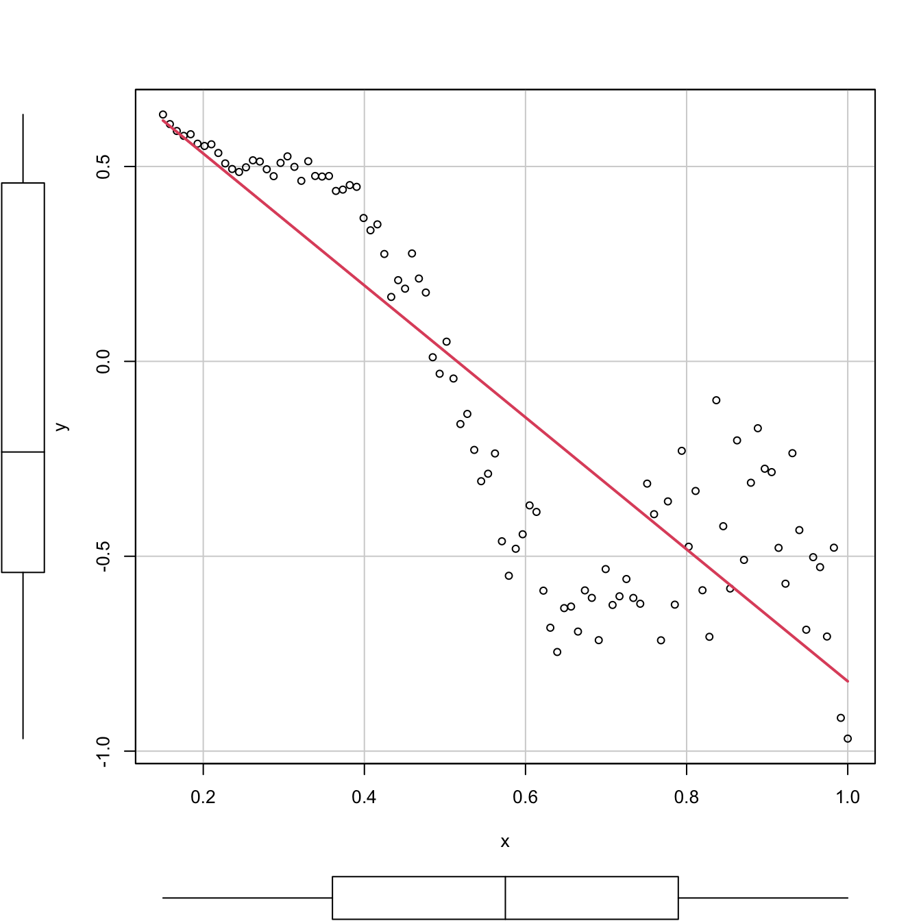

Figure 2.18: Regression line for a dataset that clearly violates the linearity and homoscedasticity assumptions. The $R^2$ is, nevertheless, as high as (approximately) $0.77.$

# Multiple linear model

# Create data that:
# 1) does not follow a linear model
# 2) the error is heteroscedastic
x1 <- seq(0.15, 1, l = 100)
set.seed(123456)
x2 <- runif(100, -3, 3)
eps <- rnorm(n = 100, sd = 0.25 * x1^2)
y <- 1 - 3 * x1 * (1 + 0.25 * sin(4 * pi * x1)) + 0.25 * cos(x2) + eps

# Great R^2!?
reg <- lm(y ~ x1 + x2)
summary(reg)
## 
## Call:
## lm(formula = y ~ x1 + x2)
## 
## Residuals:
##      Min       1Q   Median       3Q      Max 
## -0.78737 -0.20946  0.01031  0.19652  1.05351 
## 
## Coefficients:
##              Estimate Std. Error t value Pr(>|t|)    
## (Intercept)  0.788812   0.096418   8.181  1.1e-12 ***
## x1          -2.540073   0.154876 -16.401  < 2e-16 ***
## x2           0.002283   0.020954   0.109    0.913    
## ---
## Signif. codes:  0 '***' 0.001 '**' 0.01 '*' 0.05 '.' 0.1 ' ' 1
## 
## Residual standard error: 0.3754 on 97 degrees of freedom
## Multiple R-squared:  0.744,  Adjusted R-squared:  0.7388 
## F-statistic:   141 on 2 and 97 DF,  p-value: < 2.2e-16

We can visualize the fit of the latter multiple linear model, since we are in $p=2.$

# But prediction is obviously problematic
car::scatter3d(y ~ x1 + x2, fit = "linear")
rgl::rglwidget()

The previous counterexamples illustrate that a large $R^2$ means nothing in terms of inference if the assumptions of the model do not hold.

Remember that:

• $R^2$ does not measure the correctness of a linear model but its usefulness, assuming the model is correct.
• $R^2$ is the proportion of variance of $Y$ explained by $X_1,\ldots,X_p$ but, of course, only when the linear model is correct.

We finalize by pointing out a nice connection between the $R^2,$ the ANOVA decomposition, and the least squares estimator $\hat{\boldsymbol{\beta}}.$

The ANOVA decomposition gives another view on the least-squares estimates: $\hat{\boldsymbol{\beta}}$ are the estimated coefficients that maximize the $R^2$ (among all the possible estimates we could think about). To see this, recall that

$$\begin{align*} R^2=\frac{\text{SSR}}{\text{SST}}=\frac{\text{SST} - \text{SSE}}{\text{SST}}=\frac{\text{SST} - \text{RSS}(\hat{\boldsymbol{\beta}})}{\text{SST}}. \end{align*}$$

Then, if $\text{RSS}(\hat{\boldsymbol{\beta}})=\min_{\boldsymbol{\beta}\in\mathbb{R}^{p+1}}\text{RSS}(\boldsymbol{\beta}),$ then $R^2$ is maximal for $\hat{\boldsymbol{\beta}}.$

2.7.2 The $R^2\!{}_{\text{Adj}}$

As we saw, these are equivalent forms for $R^2$:

$$\begin{align} R^2=&\,\frac{\text{SSR}}{\text{SST}}=\frac{\text{SST}-\text{SSE}}{\text{SST}}=1-\frac{\text{SSE}}{\text{SST}}\nonumber\\ =&\,1-\frac{\hat\sigma^2}{\text{SST}}\times(n-p-1).\tag{2.23} \end{align}$$

The SSE on the numerator always decreases as more predictors are added to the model, even if these are not significant. As a consequence, the $R^2$ always increases with $p$. Why is this so? Intuitively, because the complexity – hence the flexibility – of the model increases when we use more predictors to explain $Y.$ Mathematically, because when $p$ approaches $n-1$ the second term in (2.23) is reduced and, as a consequence, $R^2$ grows.

The adjusted $R^2$, $R^2_\text{Adj},$ is an important quantity specifically designed to overcome this $R^2$’s flaw, ubiquitous in multiple linear regression. The purpose is to have a better tool for comparing models without systematically favoring more complex models.⁴⁸ This alternative coefficient is defined as

$$\begin{align} R^2_{\text{Adj}}:=&\,1-\frac{\text{SSE}/(n-p-1)}{\text{SST}/(n-1)}=1-\frac{\text{SSE}}{\text{SST}}\times\frac{n-1}{n-p-1}\nonumber\\ =&\,1-\frac{\hat\sigma^2}{\text{SST}}\times (n-1).\tag{2.24} \end{align}$$

The $R^2_{\text{Adj}}$ is independent of $p,$ at least explicitly. If $p=1$ then $R^2_{\text{Adj}}$ is almost $R^2$ (practically identical if $n$ is large). Both (2.23) and (2.24) are quite similar except for the last factor, which in the latter does not depend on $p.$ Therefore, (2.24) will only increase if $\hat\sigma^2$ is reduced with $p;$ in other words, if the new variables contribute in the reduction of variability around the regression plane.

The different behavior between $R^2$ and $R^2_\text{Adj}$ can be visualized with the following simulation study. Suppose that we generate a random dataset $\{(X_{i1},X_{i2},Y_i)\}_{i=1}^n,$ with $n=200$ observations of two predictors $X_1$ and $X_2$ that are distributed as a $\mathcal{N}(0,1),$ and a response $Y$ generated by the linear model

$$\begin{align} Y_i=\beta_0+\beta_1X_{i1}+\beta_2X_{i2}+\varepsilon_i,\tag{2.25} \end{align}$$

where $\varepsilon_i\sim\mathcal{N}(0,9).$ To this data, we add $196$ “garbage” predictors $X_j\sim\mathcal{N}(0,1)$ that are completely independent from $Y.$ Therefore, we end up with $p=198$ predictors where only the first two ones are relevant for explaining $Y.$ We compute now the $R^2(j)$ and $R^2_\text{Adj}(j)$ for the models

$$\begin{align} Y=\beta_0+\beta_1X_{1}+\cdots+\beta_jX_{j}+\varepsilon,\tag{2.26} \end{align}$$

with $j=1,\ldots,p,$ and we plot them as the curves $(j,R^2(j))$ and $(j,R_\text{Adj}^2(j)).$ Since $R^2$ and $R^2_\text{Adj}$ are random variables, we repeat this procedure $M=500$ times to have an idea of the variability behind $R^2$ and $R^2_\text{Adj}.$ Figure 2.19 contains the results of this experiment.

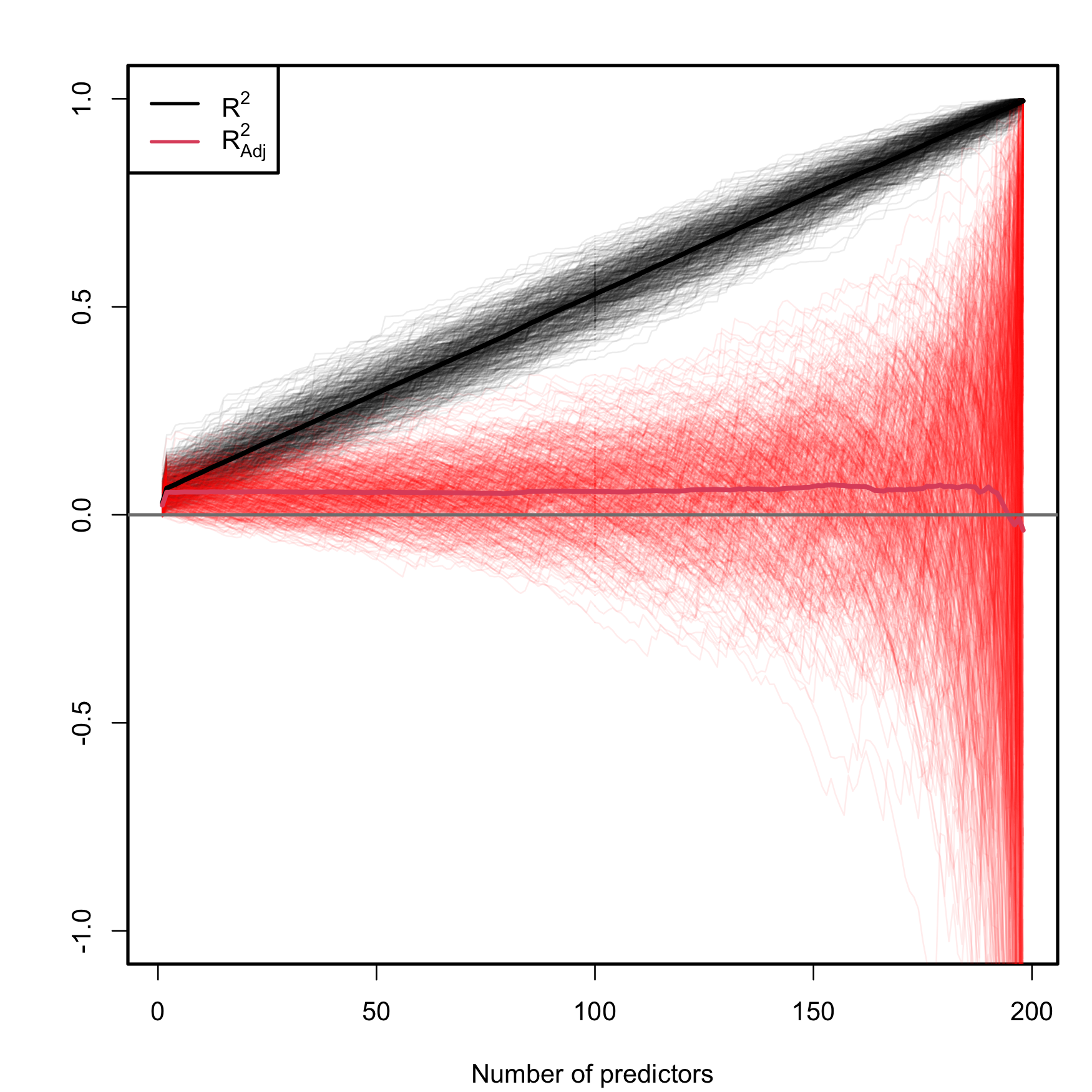
Figure 2.19: Comparison of $R^2$ and $R^2_{\text{Adj}}$ on the model (2.26) fitted with data generated by (2.25). The number of predictors $p$ ranges from $1$ to $198,$ with only the first two predictors being significant. The $M=500$ curves for each color arise from $M$ simulated datasets of sample size $n=200.$ The thicker curves are the mean of each color’s curves.

As it can be seen, the $R^2$ increases linearly with the number of predictors considered, although only the first two ones were actually relevant. Thus, if we did not know about the random mechanism (2.25) that generated $Y,$ we would be tempted to believe that the more adequate models would be the ones with a larger number of predictors. On the contrary, $R^2_\text{Adj}$ only increases in the first two variables and then exhibits a mild decaying trend, indicating that, on average, the best choice for the number of predictors is actually close to $p=2.$ However, note that $R^2_\text{Adj}$ has a huge variability when $p$ approaches $n-2,$ a consequence of the explosive variance of $\hat\sigma^2$ in that degenerate case⁴⁹. The experiment helps to visualize that $R^2_\text{Adj}$ is more adequate than the $R^2$ for evaluating the fit of a multiple linear regression⁵⁰.

An example of a simulated dataset considered in the experiment of Figure 2.19 is:

# Generate data
p <- 198
n <- 200
set.seed(3456732)
beta <- c(0.5, -0.5, rep(0, p - 2))
X <- matrix(rnorm(n * p), nrow = n, ncol = p)
Y <- drop(X %*% beta + rnorm(n, sd = 3))
data <- data.frame(y = Y, x = X)

# Regression on the two meaningful predictors
summary(lm(y ~ x.1 + x.2, data = data))

# Adding 20 "garbage" variables
# R^2 increases and adjusted R^2 decreases
summary(lm(y ~ X[, 1:22], data = data))

Implement the simulation study behind Figure 2.19 in order to replicate it.

The $R^2_\text{Adj}$ no longer measures the proportion of variation of $Y$ explained by the regression, but the result of correcting this proportion by the number of predictors employed. As a consequence of this, $R^2_\text{Adj}\leq1$ and $R^2_\text{Adj}$ can be negative.

The next code illustrates a situation where we have two predictors completely independent from the response. The fitted model has a negative $R^2_\text{Adj}.$

# Three independent variables
set.seed(234599)
x1 <- rnorm(100)
x2 <- rnorm(100)
y <- 1 + rnorm(100)

# Negative adjusted R^2
summary(lm(y ~ x1 + x2))
## 
## Call:
## lm(formula = y ~ x1 + x2)
## 
## Residuals:
##     Min      1Q  Median      3Q     Max 
## -3.5081 -0.5021 -0.0191  0.5286  2.4750 
## 
## Coefficients:
##             Estimate Std. Error t value Pr(>|t|)    
## (Intercept)  0.97024    0.10399   9.330 3.75e-15 ***
## x1           0.09003    0.10300   0.874    0.384    
## x2          -0.05253    0.11090  -0.474    0.637    
## ---
## Signif. codes:  0 '***' 0.001 '**' 0.01 '*' 0.05 '.' 0.1 ' ' 1
## 
## Residual standard error: 1.034 on 97 degrees of freedom
## Multiple R-squared:  0.009797,   Adjusted R-squared:  -0.01062 
## F-statistic: 0.4799 on 2 and 97 DF,  p-value: 0.6203

For the previous example, construct more predictors (x3, x4, …) that are independent from y. Then check that, when the predictors are added to the model, the $R^2_\text{Adj}$ decreases and the $R^2$ increases.

Beware of the $R^2$ and $R^2_\text{Adj}$ for model fits with no intercept! If the linear model is fitted with no intercept, the summary function silently returns a ‘Multiple R-squared’ and an ‘Adjusted R-squared’ that do not correspond (see this question in the R FAQ) with the seen expressions

$$\begin{align*} R^2=1-\frac{\text{SSE}}{\sum_{i=1}^n(Y_i-\bar{Y})^2},\quad R^2_{\text{Adj}}=1-\frac{\text{SSE}}{\text{SST}}\times\frac{n-1}{n-p-1}. \end{align*}$$

In the case with no intercept, summary rather returns

$$\begin{align*} R^2_0 :=1-\frac{\text{SSE}}{\sum_{i=1}^nY_i^2},\quad R^2_{0,\text{Adj}} :=1-\frac{\text{SSE}}{\sum_{i=1}^nY_i^2}\times\frac{n-1}{n-p-1}. \end{align*}$$

The reason is perhaps shocking: if the model is fitted without intercept and neither the response nor the predictors are centered, then the ANOVA decomposition does not hold, in the sense that

$$\begin{align*} \mathrm{SST} \neq \mathrm{SSR} + \mathrm{SSE}. \end{align*}$$

The fact that the ANOVA decomposition does not hold for no-intercept models has serious consequences on the theory we built. In particular, the $R^2$ can be negative and $R^2\neq r^2_{y\hat y},$ both deriving from the fact that $\sum_{i=1}^n\hat\varepsilon_i\neq0.$ Therefore, the $R^2$ cannot be regarded as the “proportion of variance explained” if the model fit is performed without intercept. The $R^2_0$ and $R^2_{0,\text{Adj}}$ versions are considered because they are the ones that arise from the “no-intercept ANOVA decomposition”

$$\begin{align*} \mathrm{SST}_0 = \mathrm{SSR}_0 + \mathrm{SSE},\quad \mathrm{SST}_0:=\sum_{i=1}^nY_i^2,\quad \mathrm{SSR}_0:=\sum_{i=1}^n\hat{Y}_i^2. \end{align*}$$

and therefore the $R^2_0$ is guaranteed to be a quantity in $[0,1].$ It would indeed be the proportion of variance explained if the predictors and the response were centered (i.e., if $\bar Y=0$ and $\bar X_j=0,$ $j=1,\ldots,p$).

The next chunk of code illustrates these concepts for the iris dataset.

# Model with intercept
mod1 <- lm(Sepal.Length ~ Petal.Width, data = iris)
mod1
## 
## Call:
## lm(formula = Sepal.Length ~ Petal.Width, data = iris)
## 
## Coefficients:
## (Intercept)  Petal.Width  
##      4.7776       0.8886

# Model without intercept
mod0 <- lm(Sepal.Length ~ 0 + Petal.Width, data = iris)
mod0
## 
## Call:
## lm(formula = Sepal.Length ~ 0 + Petal.Width, data = iris)
## 
## Coefficients:
## Petal.Width  
##       3.731

# Recall the different way of obtaining the estimators
X1 <- cbind(1, iris$Petal.Width)
X0 <- cbind(iris$Petal.Width) # No column of ones!
Y <- iris$Sepal.Length
betaHat1 <- solve(crossprod(X1)) %*% t(X1) %*% Y
betaHat0 <- solve(crossprod(X0)) %*% t(X0) %*% Y
betaHat1
##           [,1]
## [1,] 4.7776294
## [2,] 0.8885803
betaHat0
##          [,1]
## [1,] 3.731485

# Summaries: higher R^2 for the model with no intercept!?
summary(mod1)
## 
## Call:
## lm(formula = Sepal.Length ~ Petal.Width, data = iris)
## 
## Residuals:
##      Min       1Q   Median       3Q      Max 
## -1.38822 -0.29358 -0.04393  0.26429  1.34521 
## 
## Coefficients:
##             Estimate Std. Error t value Pr(>|t|)    
## (Intercept)  4.77763    0.07293   65.51   <2e-16 ***
## Petal.Width  0.88858    0.05137   17.30   <2e-16 ***
## ---
## Signif. codes:  0 '***' 0.001 '**' 0.01 '*' 0.05 '.' 0.1 ' ' 1
## 
## Residual standard error: 0.478 on 148 degrees of freedom
## Multiple R-squared:  0.669,  Adjusted R-squared:  0.6668 
## F-statistic: 299.2 on 1 and 148 DF,  p-value: < 2.2e-16
summary(mod0)
## 
## Call:
## lm(formula = Sepal.Length ~ 0 + Petal.Width, data = iris)
## 
## Residuals:
##     Min      1Q  Median      3Q     Max 
## -3.1556 -0.3917  1.0625  3.8537  5.0537 
## 
## Coefficients:
##             Estimate Std. Error t value Pr(>|t|)    
## Petal.Width    3.732      0.150   24.87   <2e-16 ***
## ---
## Signif. codes:  0 '***' 0.001 '**' 0.01 '*' 0.05 '.' 0.1 ' ' 1
## 
## Residual standard error: 2.609 on 149 degrees of freedom
## Multiple R-squared:  0.8058, Adjusted R-squared:  0.8045 
## F-statistic: 618.4 on 1 and 149 DF,  p-value: < 2.2e-16

# Wait a moment... let's see the actual fit
plot(Sepal.Length ~ Petal.Width, data = iris)
abline(mod1, col = 2) # Obviously, much better
abline(mod0, col = 3)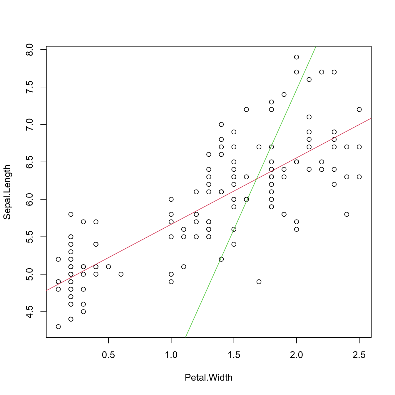

# Compute the R^2 manually for mod1
SSE1 <- sum(mod1$residuals^2)
SST1 <- sum((mod1$model$Sepal.Length - mean(mod1$model$Sepal.Length))^2)
1 - SSE1 / SST1
## [1] 0.6690277

# Compute the R^2 manually for mod0
SSE0 <- sum(mod0$residuals^2)
SST0 <- sum((mod0$model$Sepal.Length - mean(mod0$model$Sepal.Length))^2)
1 - SSE0 / SST0
## [1] -8.926872
# It is negative!

# Recall that the mean of the residuals is not zero!
mean(mod0$residuals)
## [1] 1.368038

# What summary really returns if there is no intercept
n <- nrow(iris)
p <- 1
R0 <- 1 - sum(mod0$residuals^2) / sum(mod0$model$Sepal.Length^2)
R0Adj <- 1 - sum(mod0$residuals^2) / sum(mod0$model$Sepal.Length^2) *
  (n - 1) / (n - p - 1)
R0
## [1] 0.8058497
R0Adj
## [1] 0.8045379

# What if we centered the data previously?
irisCen <- data.frame(scale(iris[, -5], center = TRUE, scale = FALSE))
modCen1 <- lm(Sepal.Length ~ Petal.Width, data = irisCen)
modCen0 <- lm(Sepal.Length ~ 0 + Petal.Width, data = irisCen)

# No problem, "correct" R^2
summary(modCen1)
## 
## Call:
## lm(formula = Sepal.Length ~ Petal.Width, data = irisCen)
## 
## Residuals:
##      Min       1Q   Median       3Q      Max 
## -1.38822 -0.29358 -0.04393  0.26429  1.34521 
## 
## Coefficients:
##               Estimate Std. Error t value Pr(>|t|)    
## (Intercept) -9.050e-16  3.903e-02     0.0        1    
## Petal.Width  8.886e-01  5.137e-02    17.3   <2e-16 ***
## ---
## Signif. codes:  0 '***' 0.001 '**' 0.01 '*' 0.05 '.' 0.1 ' ' 1
## 
## Residual standard error: 0.478 on 148 degrees of freedom
## Multiple R-squared:  0.669,  Adjusted R-squared:  0.6668 
## F-statistic: 299.2 on 1 and 148 DF,  p-value: < 2.2e-16
summary(modCen0)
## 
## Call:
## lm(formula = Sepal.Length ~ 0 + Petal.Width, data = irisCen)
## 
## Residuals:
##      Min       1Q   Median       3Q      Max 
## -1.38822 -0.29358 -0.04393  0.26429  1.34521 
## 
## Coefficients:
##             Estimate Std. Error t value Pr(>|t|)    
## Petal.Width   0.8886     0.0512   17.36   <2e-16 ***
## ---
## Signif. codes:  0 '***' 0.001 '**' 0.01 '*' 0.05 '.' 0.1 ' ' 1
## 
## Residual standard error: 0.4764 on 149 degrees of freedom
## Multiple R-squared:  0.669,  Adjusted R-squared:  0.6668 
## F-statistic: 301.2 on 1 and 149 DF,  p-value: < 2.2e-16

# But only if we center predictor and response...
summary(lm(iris$Sepal.Length ~ 0 + irisCen$Petal.Width))
## 
## Call:
## lm(formula = iris$Sepal.Length ~ 0 + irisCen$Petal.Width)
## 
## Residuals:
##    Min     1Q Median     3Q    Max 
##  4.455  5.550  5.799  6.108  7.189 
## 
## Coefficients:
##                     Estimate Std. Error t value Pr(>|t|)
## irisCen$Petal.Width   0.8886     0.6322   1.406    0.162
## 
## Residual standard error: 5.882 on 149 degrees of freedom
## Multiple R-squared:  0.01308,    Adjusted R-squared:  0.006461 
## F-statistic: 1.975 on 1 and 149 DF,  p-value: 0.1619

Let’s play the evil practitioner and try to modify the $R_0^2$ returned by summary when the intercept is excluded. If we were really evil, we could use this knowledge to fool someone that is not aware of the difference between $R_0^2$ and $R^2$ into believing that any given model is incredibly good or bad in terms of the $R^2$!

1. For the previous example, display the $R_0^2$ as a function of a shift in mean of the predictor Petal.Width. What can you conclude? Hint: you may use I() for performing the shifting inside the model equation.
2. What shift on Petal.Width would be necessary to achieve an $R_0^2\approx0.95$? Is this shift unique?
3. Do the same but for a shift in the mean of the response Sepal.Length. What shift would be necessary to achieve an $R_0^2\approx0.50$? Is there a single shift?
4. Consider the multiple linear model medv ~ nox + rm for the Boston dataset. We want to tweak the $R_0^2$ to set it to any number in $[0,1].$ Can we achieve this by only shifting rm or medv (only one of them)?
5. Explore systematically the $R_0^2$ for the shifting combinations of rm and medv and obtain a combination that delivers an $R_0^2\approx 0.30.$ Hint: use filled.contour() for visualizing the $R_0^2$ surface.

2.7.3 Case study application

Coming back to the case study, we have studied so far three models:

# Fit models
modWine1 <- lm(Price ~ ., data = wine)
modWine2 <- lm(Price ~ . - FrancePop, data = wine)
modWine3 <- lm(Price ~ Age + WinterRain, data = wine)

# Summaries
summary(modWine1)
## 
## Call:
## lm(formula = Price ~ ., data = wine)
## 
## Residuals:
##      Min       1Q   Median       3Q      Max 
## -0.46541 -0.24133  0.00413  0.18974  0.52495 
## 
## Coefficients:
##               Estimate Std. Error t value Pr(>|t|)    
## (Intercept) -2.343e+00  7.697e+00  -0.304  0.76384    
## WinterRain   1.153e-03  4.991e-04   2.311  0.03109 *  
## AGST         6.144e-01  9.799e-02   6.270 3.22e-06 ***
## HarvestRain -3.837e-03  8.366e-04  -4.587  0.00016 ***
## Age          1.377e-02  5.821e-02   0.237  0.81531    
## FrancePop   -2.213e-05  1.268e-04  -0.175  0.86313    
## ---
## Signif. codes:  0 '***' 0.001 '**' 0.01 '*' 0.05 '.' 0.1 ' ' 1
## 
## Residual standard error: 0.293 on 21 degrees of freedom
## Multiple R-squared:  0.8278, Adjusted R-squared:  0.7868 
## F-statistic: 20.19 on 5 and 21 DF,  p-value: 2.232e-07
summary(modWine2)
## 
## Call:
## lm(formula = Price ~ . - FrancePop, data = wine)
## 
## Residuals:
##      Min       1Q   Median       3Q      Max 
## -0.46024 -0.23862  0.01347  0.18601  0.53443 
## 
## Coefficients:
##               Estimate Std. Error t value Pr(>|t|)    
## (Intercept) -3.6515703  1.6880876  -2.163  0.04167 *  
## WinterRain   0.0011667  0.0004820   2.420  0.02421 *  
## AGST         0.6163916  0.0951747   6.476 1.63e-06 ***
## HarvestRain -0.0038606  0.0008075  -4.781 8.97e-05 ***
## Age          0.0238480  0.0071667   3.328  0.00305 ** 
## ---
## Signif. codes:  0 '***' 0.001 '**' 0.01 '*' 0.05 '.' 0.1 ' ' 1
## 
## Residual standard error: 0.2865 on 22 degrees of freedom
## Multiple R-squared:  0.8275, Adjusted R-squared:  0.7962 
## F-statistic: 26.39 on 4 and 22 DF,  p-value: 4.057e-08
summary(modWine3)
## 
## Call:
## lm(formula = Price ~ Age + WinterRain, data = wine)
## 
## Residuals:
##      Min       1Q   Median       3Q      Max 
## -0.88964 -0.51421 -0.00066  0.43103  1.06897 
## 
## Coefficients:
##              Estimate Std. Error t value Pr(>|t|)    
## (Intercept) 5.9830427  0.5993667   9.982 5.09e-10 ***
## Age         0.0360559  0.0137377   2.625   0.0149 *  
## WinterRain  0.0007813  0.0008780   0.890   0.3824    
## ---
## Signif. codes:  0 '***' 0.001 '**' 0.01 '*' 0.05 '.' 0.1 ' ' 1
## 
## Residual standard error: 0.5769 on 24 degrees of freedom
## Multiple R-squared:  0.2371, Adjusted R-squared:  0.1736 
## F-statistic:  3.73 on 2 and 24 DF,  p-value: 0.03884

The model modWine2 has the largest $R^2_\text{Adj}$ among the three studied. It is a model that explains the $82.75\%$ of the variability in a non-redundant way and with all its coefficients significant. Therefore, we have a formula for effectively explaining and predicting the quality of a vintage (answers Q1). Prediction and, importantly, quantification of the uncertainty in the prediction, can be done through the predict function.

Furthermore, the interpretation of modWine2 agrees with well-known facts in viticulture that make perfect sense. Precisely (answers Q2):

• Higher temperatures are associated with better quality (higher priced) wine.
• Rain before the growing season is good for the wine quality, but during harvest is bad.
• The quality of the wine improves with the age.

Although these conclusions could be regarded as common folklore, keep in mind that this model

• allows to quantify the effect of each variable on the wine quality and
• provides a precise way of predicting the quality of future vintages.

---

46. Which is not the $\hat\sigma^2$ in (2.21), but $\hat\sigma^2$ is obviously dependent on $\sigma^2.$↩︎

47. Which do not hold!↩︎

48. An informal way of regarding the difference between $R^2$ and $R^2_\text{Adj}$ is by thinking of $R^2$ as a measure of fit that “is not aware of the dangers of overfitting”. In this interpretation, $R^2_\text{Adj}$ is the overfitting-aware version of $R^2.$↩︎

49. This indicates that $R^2_\text{Adj}$ can act as a model selection device up to a certain point, as its effectiveness becomes too variable, too erratic, when the number of predictors is very high in comparison with $n.$↩︎

50. Coincidentally, the experiment also serves as a reminder about the randomness of $R^2$ and $R^2_{\text{Adj}},$ a fact that is sometimes overlooked.↩︎