10.7 $2\times 2$ Contingency Table in Practice

Let us focus on attribute $k$. For an element $p_{ab}$ in the table,

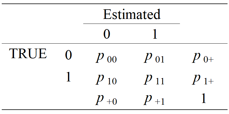
$$\begin{aligned} p_{ab}&=P(\alpha_k=a,\hat{\alpha}_k(\mathbf{Y})=b)\\ &=P(\alpha_k=a,\hat{\alpha}_k(\mathbf{Y})=b|\mathbf{Y})P(\mathbf{Y}) \end{aligned}$$ Given a finite sample $\mathbf{y}$ of size $n$, we can estimate

$$\begin{aligned} \hat{p}_{ab}&=P(\alpha_k=a,\hat{\alpha}_k(\mathbf{Y}=\mathbf{y})=b)\\ &=P(\alpha_k=a,\hat{\alpha}_k(\mathbf{Y}=\mathbf{y})=b|\mathbf{Y}=\mathbf{y})P(\mathbf{Y}=\mathbf{y})\\ &=\frac{1}{n}\sum_{i=1}^n\underbrace{P(\alpha_{ik}=a|\mathbf{y}_i)}_{\text{estimated probability of mastery/non-mastery}}\underbrace{I(\hat{\alpha}_{ik}=b|\mathbf{y}_i)}_{\text{estimated mastery status}}\\ \end{aligned}$$ in this case, we are calclluating the joint probability that the true mastery status of attribute $k$ is $a$ (either 1 for mastery or 0 for non-mastery) and the model estimated mastery as $b$ (either 0 or 1). $P(\alpha_k=a|Y=y)$ is the probability of true mastery or non-mastery for attribute $k$ given the response pattern $Y=y$. $P(\hat{\alpha}_k(Y=y)=b|Y=y)$ is the probability that the model’s estimate of mastery is $b$ given the response pattern $Y=y$.

Lest us focus on two probabilities:

• $P\left(\alpha_{i k}=a \mid \mathbf{y}_i\right)$ is the posterior probability that individual $i$ has mastery(or non-mastery) of attribute $k$, given their response vector $y_i$.

• $I\left(\hat{\alpha}_{i k}=b \mid \mathbf{y}_i\right)$ is an indicator function that is 1 if the model estimates the mastery status $b$ correctly, and 0 otherwise.