4.8 Estimation of A combination of models

To estimate different models for different items, call GDINA function again and specify the data and Q-matrix as the first two arguments.

Note that we can also impose the monotonic constraints by setting mono.constraint = TRUE.

Code

models <- c(rep("GDINA", 5), "DINA", "DINO", "ACDM", "LLM", "RRUM", "DINA",
    "DINO", "ACDM", "LLM", "RRUM")
fit4 <- GDINA(dat = data1, Q = Q1, model = models, verbose = 0, mono.constraint = TRUE)

To print some general model estimation information, type fit4 in Rstudio console:

Code

fit4

## Call:
## GDINA(dat = data1, Q = Q1, model = models, mono.constraint = TRUE, 
##     verbose = 0)
## 
## GDINA version 2.9.3 (2022-08-13) 
## ===============================================
## Data
## -----------------------------------------------
## # of individuals    groups    items         
##              837         1       15
## ===============================================
## Model
## -----------------------------------------------
## Fitted model(s)       = GDINA DINA DINO ACDM LLM RRUM 
## Attribute structure   = saturated 
## Attribute level       = Dichotomous 
## ===============================================
## Estimation
## -----------------------------------------------
## Number of iterations  = 89 
## 
## For the final iteration:
##   Max abs change in item success prob. = 0.0001 
##   Max abs change in mixing proportions = 0.0000 
##   Change in -2 log-likelihood          = 0.0003 
##   Converged?                           = TRUE 
## 
## Time used             = 1.2 secs

To extract item parameters, we can use coef function, as in

Code

coef(fit4)

## $`Item 1`
## P(0) P(1) 
## 0.94 0.99 
## 
## $`Item 2`
## P(0) P(1) 
## 0.38 0.86 
## 
## $`Item 3`
## P(0) P(1) 
## 0.54 0.81 
## 
## $`Item 4`
## P(0) P(1) 
## 0.54 0.92 
## 
## $`Item 5`
## P(00) P(10) P(01) P(11) 
##  0.35  0.74  0.64  0.92 
## 
## $`Item 6`
## P(00) P(10) P(01) P(11) 
##  0.24  0.24  0.24  0.85 
## 
## $`Item 7`
##  P(00)  P(10)  P(01)  P(11) 
## 0.0019 0.7193 0.7193 0.7193 
## 
## $`Item 8`
## P(00) P(10) P(01) P(11) 
##  0.20  0.64  0.35  0.80 
## 
## $`Item 9`
## P(00) P(10) P(01) P(11) 
##  0.16  0.45  0.35  0.70 
## 
## $`Item 10`
## P(00) P(10) P(01) P(11) 
##  0.36  0.70  0.39  0.76 
## 
## $`Item 11`
## P(00) P(10) P(01) P(11) 
##  0.67  0.67  0.67  0.92 
## 
## $`Item 12`
## P(00) P(10) P(01) P(11) 
##  0.15  0.57  0.57  0.57 
## 
## $`Item 13`
## P(00) P(10) P(01) P(11) 
##  0.15  0.34  0.43  0.62 
## 
## $`Item 14`
## P(000) P(100) P(010) P(001) P(110) P(101) P(011) P(111) 
##   0.19   0.54   0.29   0.19   0.67   0.54   0.29   0.67 
## 
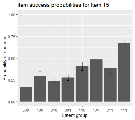
## $`Item 15`
## P(000) P(100) P(010) P(001) P(110) P(101) P(011) P(111) 
##   0.17   0.29   0.23   0.28   0.41   0.48   0.38   0.67

To obtain delta parameters, specify what = “delta”:

Code

coef(fit4, what = "delta")

## $`Item 1`
##   d0   d1 
## 0.94 0.05 
## 
## $`Item 2`
##   d0   d1 
## 0.38 0.48 
## 
## $`Item 3`
##   d0   d1 
## 0.54 0.27 
## 
## $`Item 4`
##   d0   d1 
## 0.54 0.39 
## 
## $`Item 5`
##    d0    d1    d2   d12 
##  0.35  0.39  0.28 -0.11 
## 
## $`Item 6`
##   d0   d1 
## 0.24 0.62 
## 
## $`Item 7`
##     d0     d1 
## 0.0019 0.7173 
## 
## $`Item 8`
##   d0   d1   d2 
## 0.20 0.45 0.16 
## 
## $`Item 9`
##   d0   d1   d2 
## -1.7  1.5  1.0 
## 
## $`Item 10`
##    d0    d1    d2 
## -1.03  0.67  0.08 
## 
## $`Item 11`
##   d0   d1 
## 0.67 0.25 
## 
## $`Item 12`
##   d0   d1 
## 0.15 0.42 
## 
## $`Item 13`
##   d0   d1   d2 
## 0.15 0.19 0.28 
## 
## $`Item 14`
##    d0    d1    d2    d3 
## -1.44  1.62  0.54  0.00 
## 
## $`Item 15`
##    d0    d1    d2    d3 
## -1.79  0.56  0.33  0.51

We can still draw the IRF plot of item 15, using the following code:

Code

plot(fit4, what = "IRF", item = c(15), withSE = TRUE)

To obtain attribute estimates, use the function personparm:

Code

head(personparm(fit4))

##      A1 A2 A3
## [1,]  0  1  1
## [2,]  0  0  1
## [3,]  1  1  0
## [4,]  0  1  0
## [5,]  0  0  0
## [6,]  1  1  0