4.6 ACDM estimation

To estimate the ACDM, call GDINA function again and specify the data and Q-matrix as the first two arguments.

Code

#Fit the data using ACDM
fit3 <- GDINA(dat = data1, Q = Q1,model = "ACDM", verbose = 0)

To print some general model estimation information, type fit3 in Rstudio console:

Code

fit3

## Call:
## GDINA(dat = data1, Q = Q1, model = "ACDM", verbose = 0)
## 
## GDINA version 2.9.3 (2022-08-13) 
## ===============================================
## Data
## -----------------------------------------------
## # of individuals    groups    items         
##              837         1       15
## ===============================================
## Model
## -----------------------------------------------
## Fitted model(s)       = ACDM 
## Attribute structure   = saturated 
## Attribute level       = Dichotomous 
## ===============================================
## Estimation
## -----------------------------------------------
## Number of iterations  = 70 
## 
## For the final iteration:
##   Max abs change in item success prob. = 0.0001 
##   Max abs change in mixing proportions = 0.0001 
##   Change in -2 log-likelihood          = 0.0004 
##   Converged?                           = TRUE 
## 
## Time used             = 0.6276 secs

To extract item parameters, we can use coef function, as in

Code

coef(fit3)

## $`Item 1`
## P(0) P(1) 
## 0.94 0.98 
## 
## $`Item 2`
## P(0) P(1) 
## 0.24 0.82 
## 
## $`Item 3`
## P(0) P(1) 
## 0.54 0.81 
## 
## $`Item 4`
## P(0) P(1) 
## 0.47 0.87 
## 
## $`Item 5`
## P(00) P(10) P(01) P(11) 
##  0.29  0.69  0.56  0.96 
## 
## $`Item 6`
## P(00) P(10) P(01) P(11) 
## 0.086 0.519 0.312 0.745 
## 
## $`Item 7`
## P(00) P(10) P(01) P(11) 
## 0.057 0.416 0.473 0.831 
## 
## $`Item 8`
## P(00) P(10) P(01) P(11) 
## 0.082 0.625 0.287 0.830 
## 
## $`Item 9`
## P(00) P(10) P(01) P(11) 
##  0.06  0.40  0.33  0.68 
## 
## $`Item 10`
## P(00) P(10) P(01) P(11) 
##  0.37  0.72  0.38  0.74 
## 
## $`Item 11`
## P(00) P(10) P(01) P(11) 
##  0.46  0.64  0.72  0.90 
## 
## $`Item 12`
## P(00) P(10) P(01) P(11) 
##  0.12  0.43  0.39  0.69 
## 
## $`Item 13`
## P(00) P(10) P(01) P(11) 
## 0.099 0.293 0.369 0.563 
## 
## $`Item 14`
## P(000) P(100) P(010) P(001) P(110) P(101) P(011) P(111) 
##   0.15   0.56   0.26   0.13   0.67   0.54   0.24   0.66 
## 
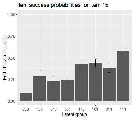
## $`Item 15`
## P(000) P(100) P(010) P(001) P(110) P(101) P(011) P(111) 
##  0.091  0.287  0.230  0.241  0.426  0.437  0.380  0.576

To obtain delta parameters, specify what = “delta”:

Code

coef(fit3, what = "delta")

## $`Item 1`
##    d0    d1 
## 0.936 0.045 
## 
## $`Item 2`
##   d0   d1 
## 0.24 0.59 
## 
## $`Item 3`
##   d0   d1 
## 0.54 0.28 
## 
## $`Item 4`
##   d0   d1 
## 0.47 0.40 
## 
## $`Item 5`
##   d0   d1   d2 
## 0.29 0.40 0.27 
## 
## $`Item 6`
##    d0    d1    d2 
## 0.086 0.433 0.226 
## 
## $`Item 7`
##    d0    d1    d2 
## 0.057 0.358 0.416 
## 
## $`Item 8`
##    d0    d1    d2 
## 0.082 0.543 0.206 
## 
## $`Item 9`
##   d0   d1   d2 
## 0.06 0.34 0.27 
## 
## $`Item 10`
##    d0    d1    d2 
## 0.367 0.353 0.017 
## 
## $`Item 11`
##   d0   d1   d2 
## 0.46 0.18 0.26 
## 
## $`Item 12`
##   d0   d1   d2 
## 0.12 0.30 0.26 
## 
## $`Item 13`
##    d0    d1    d2 
## 0.099 0.194 0.271 
## 
## $`Item 14`
##     d0     d1     d2     d3 
##  0.146  0.416  0.112 -0.019 
## 
## $`Item 15`
##    d0    d1    d2    d3 
## 0.091 0.196 0.139 0.150

We can still draw the IRF plot of item 15, using the following code:

Code

plot(fit3, what = "IRF", item = c(15), withSE = TRUE)

To obtain attribute estimates, use the function personparm:

Code

head(personparm(fit3))

##      A1 A2 A3
## [1,]  1  1  1
## [2,]  0  0  1
## [3,]  1  1  0
## [4,]  0  1  0
## [5,]  0  0  0
## [6,]  1  1  0